Style Transfer
The idea of style transfer is to re-imagine an image in a style of another image by “transferring” its “style” to the image.
The meaning of transferring and style are not obvious and probably even subjective.
One approach was developed by Gatys, 2015, where deep learning, or convolutional neural networks (CNN) were used.
The idea is relatively simple and the results are definitely appealing and match what most would consider to be a style transfer.
Here I wanted to implement it using PyTorch, following the paper and the TensorFlow tutorial.
The main innovative idea behind the style transfer method, is that the shallower (first) convolutional (conv layers (or filters) of a CNN, which was pre-trained on a large image dataset such as ImageNet, have learned useful filters to identify generic features in an image, e.g. edges, simple shapes, geometry, colors. Things that we would associate with the style of a painting for example. The deeper layers, on the other hand, since they act on the outputs of the previous layers, they are able to learn more complex features, which are useful to identify specific complex objects, such as eyes, face, etc., features which are more relevant to the actual content of the image.
Given a pre-trained network, the idea is the following:
- Choose a style image, and a content image.
- Initialise the final image with either random pixels or start with the content image.
- Run the three images through the network, and extract the intermediate features generated by the shallow conv layers as style features, and the later conv layers as content features.
- Compute the style loss associated with the generated image by comparing it with the style of the style image.
- Compute the content loss associated with the generated image by comparing it with the content of the original image.
- Combine both losses with weights and run back propagation on the generated image, and update it using gradient descent.
The final image generated by this process, will have style inspired by the style image as described by the shallow conv layers, and content matching the original image. THe main point to note here is that unlike conventional CNN related tasks where we train using an input image and a label and update the network’s weights, here the network is fixed and what is trained is the input image, the input image pixels serve as the “weights” which are updated to reduce the loss defined above.
I’ve used Google Colab to run the model, making use of the free GPU. The Google Colab notebook can be found here.
The code
Imports:
import matplotlib.pyplot as plt
import numpy as np
from PIL import Image
from tqdm import notebook

import torch
import torch.nn as nn
import torch.nn.functional as F
import torch.optim as optim
from torchvision import transforms, models
# Set device based on availability (cuda or cpu)
device = torch.device('cuda' if torch.cuda.is_available() else "cpu")
print(device)
# Load vgg19 model. Strip away the classification head, to keep only features
vgg = models.vgg19().features
The VGG model was the old style of CNN models, without skip connections, therefore it’s much shallower good enough. Composed of repeated blocks of conv, ReLU and max pooling. It has the following layers:
Sequential(
  (0): Conv2d(3, 64, kernel_size=(3, 3), stride=(1, 1), padding=(1, 1))
  (1): ReLU(inplace=True)
  (2): Conv2d(64, 64, kernel_size=(3, 3), stride=(1, 1), padding=(1, 1))
  (3): ReLU(inplace=True)
  (4): MaxPool2d(kernel_size=2, stride=2, padding=0, dilation=1, ceil_mode=False)
  (5): Conv2d(64, 128, kernel_size=(3, 3), stride=(1, 1), padding=(1, 1))
  (6): ReLU(inplace=True)
  (7): Conv2d(128, 128, kernel_size=(3, 3), stride=(1, 1), padding=(1, 1))
  (8): ReLU(inplace=True)
  (9): MaxPool2d(kernel_size=2, stride=2, padding=0, dilation=1, ceil_mode=False)
  (10): Conv2d(128, 256, kernel_size=(3, 3), stride=(1, 1), padding=(1, 1))
  (11): ReLU(inplace=True)
  (12): Conv2d(256, 256, kernel_size=(3, 3), stride=(1, 1), padding=(1, 1))
  (13): ReLU(inplace=True)
  (14): Conv2d(256, 256, kernel_size=(3, 3), stride=(1, 1), padding=(1, 1))
  (15): ReLU(inplace=True)
  (16): Conv2d(256, 256, kernel_size=(3, 3), stride=(1, 1), padding=(1, 1))
  (17): ReLU(inplace=True)
  (18): MaxPool2d(kernel_size=2, stride=2, padding=0, dilation=1, ceil_mode=False)
  (19): Conv2d(256, 512, kernel_size=(3, 3), stride=(1, 1), padding=(1, 1))
  (20): ReLU(inplace=True)
  (21): Conv2d(512, 512, kernel_size=(3, 3), stride=(1, 1), padding=(1, 1))
  (22): ReLU(inplace=True)
  (23): Conv2d(512, 512, kernel_size=(3, 3), stride=(1, 1), padding=(1, 1))
  (24): ReLU(inplace=True)
  (25): Conv2d(512, 512, kernel_size=(3, 3), stride=(1, 1), padding=(1, 1))
  (26): ReLU(inplace=True)
  (27): MaxPool2d(kernel_size=2, stride=2, padding=0, dilation=1, ceil_mode=False)
  (28): Conv2d(512, 512, kernel_size=(3, 3), stride=(1, 1), padding=(1, 1))
  (29): ReLU(inplace=True)
  (30): Conv2d(512, 512, kernel_size=(3, 3), stride=(1, 1), padding=(1, 1))
  (31): ReLU(inplace=True)
  (32): Conv2d(512, 512, kernel_size=(3, 3), stride=(1, 1), padding=(1, 1))
  (33): ReLU(inplace=True)
  (34): Conv2d(512, 512, kernel_size=(3, 3), stride=(1, 1), padding=(1, 1))
  (35): ReLU(inplace=True)
  (36): MaxPool2d(kernel_size=2, stride=2, padding=0, dilation=1, ceil_mode=False)
)
Creating the model class, inhering from PyTorch’s nn.Module:
class StyleTransfer(nn.Module):
  def __init__(self):
    super(StyleTransfer, self).__init__()

    # Choose the conv layers used for style (lower levels)
    self.style_layers = [0, 5, 10, 19, 28]

    # Choose the conv layers used for context (deeper levels). Can choose multiple, but it's custom to chose 1.
    self.content_layers = [21]

    # The vgg model, pretrained and only features (without classification head) and without the layer beyond the content last style layer
    self.model = models.vgg19(pretrained=True).features[:31]

    # In the paper the recommend swapping max pool layers with avg pool.
    for i, layer in enumerate(self.model):
      if isinstance(layer, torch.nn.MaxPool2d):
        self.model[i] = torch.nn.AvgPool2d(kernel_size=2, stride=2, padding=0)

    # The model weights are fixed, we're not gonna backprop them,
    # therefore can set their requires grad to False.
    for param in self.model.parameters():
      param.requires_grad = False


  # Define the model's forward pass
  def forward(self, image):

    # List to append the style/content features from the intermediate layers
    style_features = []
    content_features = []

    for layer_index, layer in enumerate(self.model):

      # pass the image through the layer
      image = layer(image)

      # Append the output only if it's one
      # of the predefined layers
      if layer_index in self.style_layers:
        style_features.append(image)
      elif layer_index in self.content_layers:
        content_features.append(image)

    # return dictionary with content and style
    return {'content': content_features, 'style':style_features}
Utility functions
def load_img(path_to_img):
    """
    Load image using PIL, resize it to have
    maximum dimension of 512, to reduce computation time
    """
    max_dim = 512
    image = Image.open(path_to_img)
    image.thumbnail((max_dim, max_dim))
    return image

def prepare_img(image):
    """
    Prepare image as a tensor with a batch axis, required for loading into the model.
    """

    # The normalize transform, normalizes
    # the image to using the Imagenet parameters, on which
    # VGG was trained.
    # For each channel: image -> (image - mean)/std
    loader = transforms.Compose(
      [
       transforms.ToTensor(),
       transforms.Normalize((0.485, 0.456, 0.406), (0.229, 0.224, 0.225))
      ]
    )

    # Perform transformation and add batch axis (0)
    image = loader(image).unsqueeze(0)

    # move image to the defined device
    return image.to(device)

def convert_img(image):
    """
    Convert a tensor of a batch of a single image to a numpy array
    """
    # transfer to cpu
    image = image.to('cpu').clone()

    # remove batch axis, turn from tensor to numpy array
    image = image.squeeze(0).numpy()

    # put channels at the last axis
    image = image.transpose(1, 2, 0)

    # reverse imagenet normalization
    image = image * np.array((0.229, 0.224, 0.225)) + np.array((0.485, 0.456, 0.406))

    # clip image pixes between 0 and 1
    image = np.clip(image, 0, 1)
    return image

def save_image(image, filename):
    """
    Save a numpy array with pixels in range [0,1] as an image
    """
    # To save image using PIL, need to rescale pixel values to 0 -> 255.
    rescaled = (255.0 / image.max() * (image - image.min())).astype(np.uint8)

    im = Image.fromarray(rescaled, 'RGB')

    im.save(filename)
Next we define the loss function, which the network will use to adjust it’s input image in this case, in order to reduce the total loss. The loss in this case is a combination of 2 contributions: Style loss and content loss, each defined in the functions below. When training we additionally have a weight assigned to the style loss, which will allow to have the style influence more the total loss, and therefore the resulting image.
The content loss is a simple pixel by pixels mean squared error loss, evaluated between the generated image content layer and the original image content layer.
def content_loss(input, target):
  """ Mean square error loss between image pixels """
  return F.mse_loss(input, target)
The trick in the paper is in the choice of the style loss, as it’s not obvious how to properly capture style, which is not a simple pixel by pixel difference. They used the Gram matrix, which is a form of a correlation matrix between the different channels (or features following the conv layers). The dea is that two images with similar styles will have similar Gram matrices, or similar correlations between the different feature maps generated by the style conv layers.
def gram_matrix(input):
    """
    Computes the gram matrix - the matrix of all inner products between all feature maps (channels)
    """
    # get batch, channels, height width
    b,c,h,w = input.shape

    # reshape tensor to be channels rows by (height*width) columns
    input = input.view(c, h*w)

    # matrix multiplication of reshaped image by reshaped image transpose
    result = torch.mm(input, input.t())

    # An alternative way: result = torch.einsum('bcij,bdij -> bcd', input, input)

  return result


def style_loss(input, target):
  """
  mean square error of Gram matrices
  """
  b,c,h,w = target.shape
  gr_inp = gram_matrix(input)
  gr_tar = gram_matrix(target)

  # the loss is the mean squared error between the
  # Gram matrices, with a normalization of number of pixels
  return F.mse_loss(gr_inp, gr_tar)/ (c * h * w)
As pointed out in the TensorFlow tutorial, an additional useful loss, is to avoid having sharp differences on a single pixel level, e.g. sharp edges. The suggested variation loss, allows to smooth the generated image:
def variation_loss(input):
  """
  smoothness loss, penalizes sharp edges on a one pixel scale
  """

  # neighboring pixels differences on the horizontal direction
  x_var = input[:,:,1:,:] - input[:,:,:-1,:]

  # neighboring pixels differences on the vertical direction
  y_var = input[:,:,:,1:] - input[:,:,:,:-1]

  # return the sum of absolute values as the loss
  return torch.sum(torch.abs(x_var)) + torch.sum(torch.abs(y_var))
Training loop
In the paper a random image (i.e. pixels normally distributed with mean 0 std 1) was used as the initial input. Here I use the content image as the starting point, which requires less training epochs to get a decent result.
def train(cont_img,
style_img,
epochs=500,
style_ratio=1e3,
variation_weight=1e-2,
save_intermediate=False,
save_name='gen_image'):
"""
Generates an image by transferring style (style_image_path)
to a content image (cont_image_path), with the style weight given
by style_ratio and run epoch number of iterations.
Images are saved with the name prefix.
"""
# create image loader for the model's input i.e.
# transforming to tensor and adding batch axis
cont_img = prepare_img(cont_img)
style_img = prepare_img(style_img)
# The generated image is the input image which
# we set as trainable, i.e. requiring gradient calculation
gen_img = cont_img.requires_grad_(True)
# The random alternative
# gen_img = torch.rand_like(cont_img).requires_grad_(True)
# Initialize the style transfer model and move it to the device.
# The eval command is needed to let pytorch
# know when we are using the model for evaluation and not training.
# This only controls things like batch norm and dropout,
# which we don't have in this model, but good practice
model = StyleTransfer().to(device).eval()
# Define optimizer with the learning parameters being the input image pixels and a learning lrate
optimizer = optim.Adam([gen_img], lr=0.03)
# Lists to store the epoch losses
style_losses = []
content_losses = []
tot_losses = []
# Run style and content image through model
# the detach() command, removes the passed images from the computation graph,
# as we don't need to track gradients for the operations done on them.
orig_output = model(cont_img.detach())
style_output = model(style_img.detach())
# Get content features from the content image
content_target = orig_output['content']
# Get style feature from the style image
style_target = style_output['style']
# Get number of layers for normalisation
num_style_layers = len(style_target)
# Start training
print(f"Training for {epochs} epochs, with style ratio: {style_ratio}")
for i in notebook.tqdm(range(epochs)):
# Zero the accumulated gradients
# on each iteration
optimizer.zero_grad()
# Run the input image through model
gen_output = model(gen_img)
# Get content features for the input image
gen_content = gen_output['content']
# Get style features for the input image
gen_style = gen_output['style']
# Initialize losses
style_loss_tot = 0
cont_loss_tot = 0
# Compute style loss and add it to total from each feature layer
for j, stl in enumerate(gen_style):
style_loss_tot += style_loss(stl, style_target[j])
# Normalize by number of layers
style_loss_tot /= num_style_layers
# Compute content loss (one layer)
cont_loss_tot = content_loss(gen_content[0], content_target[0])
# Compute total loss as a weighted sum of style and content loss
loss = style_ratio*style_loss_tot + cont_loss_tot
# Add variation loss
loss += variation_weight*variation_loss(gen_img)
# Perform back propagation (calculate gradients)
loss.backward()
# Make gradient descent step
optimizer.step()
# Track style, content and total loss for plotting
style_losses.append(style_ratio*style_loss_tot)
content_losses.append(cont_loss_tot)
tot_losses.append(loss)
# Optional save intermediate images
if save_intermediate:
if i%50 == 0 and i>0:
print(f"saving image {i}")
conv_img = convert_img(gen_img.detach())
save_image(conv_img, save_name + '.jpg')
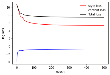
# Show loss through training process
plt.figure()
plt.plot(np.log(style_losses), label='style loss', color='red')
plt.plot(np.log(content_losses), label='content loss', color='blue')
plt.plot(np.log(tot_losses), label='Total loss', color='black')
# Show and save final image
plt.legend()
plt.figure()
conv_img = convert_img(gen_img.detach())
plt.imshow(conv_img)
print('saving final image')
save_image(conv_img, save_name+'.jpg')
Example:
Define parameters:
# These were chosen by trying what gives desired results
# There is no point going too high with the style loss, as at some point it will
# simply be the entire loss, and as we're starting from the content, it won't
# change much the final output.
epochs = 500  # number of training epochs
style_ratio = 1e3  # the style loss weight relative to content loss
content_image = "horses.jpg"
style_image = "stary_night.jpg"
save_name = "horses_stary"  # filename for the output
Load content and style images:
cont_img = load_img(content_image)
style_img = load_img(style_image)

plt.subplots(1,2, figsize=(10,8))
plt.subplot(1,2,1)
plt.imshow(cont_img)
plt.subplot(1,2,2)
plt.imshow(style_img)
Run training
train(cont_img,
    style_img,
    style_ratio=style_ratio,
    epochs=epochs,
    save_name=save_name)
Examples:
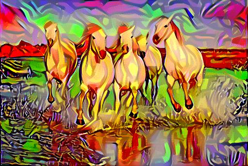
| Content Image: Horses | Style Image: Starry night by Vincent Van Gogh |
 |
 |
Result:
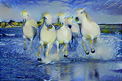
Here I used epochs=200. Training for more epochs will further reduce the loss making the image match the style more and more at the expanse of losing the content information.
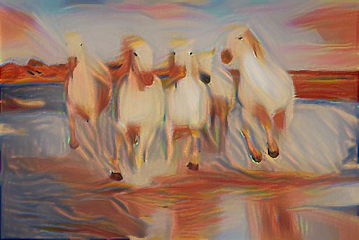
| Content Image: Horses | Style Image: The Scream by Munch |
| |
 |
Result:
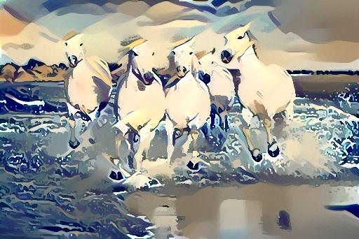
| Content Image: Horses | Style Image: The Great Wave |
| |
 |
Result:
| Content Image: Horses | Style Image: Picasso |
| |
 |
Result:
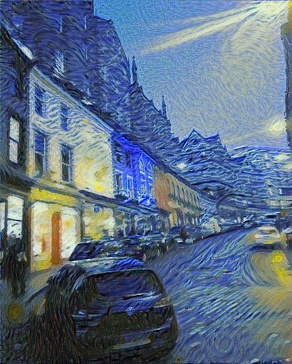
In the next example I used epochs = 1000 and style_ratio = 1e5:
| Content Image: Edinburgh | Style Image: Starry Night by Vincent Van Gogh |
 |
|
Result:
An example (log) loss curve from the training, showing that given the weights, the loss is primarily driven by the style loss: