Ant Colony Optimization
I’ve recently been interested in vehicle routing problem, a variation on the famous travelling salesperson problem (TSP), where the task is given a graph with the distances between cities, find the shortest path visiting all cities once and returning to the starting city. The problem falls under the complexity class NP-hard, which loosely means they cannot be solved in polynomial time. (Also it is not NP-complete, which means it is both in NP-Hard and in NP, where NP means that a solution can be verified in polynomial time, and for TSP verifying a path is the shortest is the same as finding the shortest path.)
Given it cannot be solved in polynomial time, as the number of cities grows, the time it would take to solve it by brute force of checking all possible paths, would grow as n! (n - number of cities). Therefore, people have looked for more optimised ways to approach the problem and get at least a “good enough solution” using what are known as meta-heuristic approaches. A very appealing approach, given its inspiration from nature, is known as the Ant Colony Optimisation (Dorigo, 1991).
The idea is very elegant and relies on nature’s long and trialed experience. Specifically, ants. Ant colonies are observed to be very organised in terms of how they self-sustain the group, finding food and bringing it back. Initially, each ant may choose a random starting path to reach its destination, however as more and more ants choose paths reach their destination and return, the ones that chose the shortest overall path, will return before the ones choosing a longer path. The key part is the information passed between the ants in the form of pheromones deposited along the path, no other more complex signal is required. The next ant when choosing a path, will be more inclined to choose the path with more pheromones, which from what I described will, with time, tend towards the shortest path, being traversed and reinforced with pheromones, leading eventually to all the ants converging on the shortest path. The elegance in this approach to me is in the emergence of global coordination through local information. An idea familiar from complex systems, and in physics was described by Phillip Anderson as “More is different”, one will not learn about this large scale coordination by reducing the ant colony to individual non-interacting ants.
Back to the travelling salesman problems, the application of the ant colony behaviour with some additional improvements, is as follows:
-
Start with ant at a given node and a small equal amount of pheromones on all edges (for stability).
-
Move the ant using a probability distribution over the allowed node given by:
where $\tau_{ij}$ is the amount of pheromone deposited on edge $ij$, and plays the role of the collective information passed by other ants, and $\eta_{ij}$ is a heuristic attractiveness of a given edge (A common choice is $\eta_{ij}\sim\frac{1}{d_{ij}}$, where $d_{ij}$ is the edge length, therefore shorter is better). The powers $\alpha$ and $\beta$ are tuning parameters for the weight of either $\tau$ or $\eta$.
The idea of having both of these terms, is similar to the famous explore-exploit trade-off, where we want the ants to exploit the information passed from other ants, while also exploring other paths through the immediate information on the available edges.
-
An optimization is to include an evaporation parameter $\rho \in [0,1]$, which allows for pheromones to evaporate, helping in avoiding the ants to converge early on a bad solution and allowing more exploration, therefore update: $\tau_{ij} \rightarrow \rho\tau_{ij}$.
-
After all ants have completed a full path, calculate the length of all path, and deposit an amount of pheromone $\Delta \tau^k_{ij} = \frac{Q}{L^k}$ on each edge $ij$ that ant $k$ went through, where $L^k$ is the total path length for ant $k$, and $Q$ is another free tuning parameter.
-
Repeat until convergence or number of iterations.
Another variation to the above, which I have used in the implementation below, is known as the “Elitist ant”, which is very cute. In this variation we additionally add an amount of pheromone $\frac{Q_e}{L^*}$ on each edge of the shortest overall path found so far in all iterations. This serves as an additional global information to guide the ants.
One of the disadvantages of the Ant system optmisation is the large number of free parameters, for which the optimal parameters depend on the particular problem or graph. Most parameters represent a balance between exploration and exploitation. The choice of parameters may determine how good of a path the ants will find. Generally, the more ants and iterations the more chance for exploration, however for relatively simpler graphs, too many ants can result in slow convergence.
Code
The code and notebook can be found in the github repo here.
class AntOpt():
    def __init__(self,
                 points,
                 d_matrix = None,
                 dist='euclid', # distance metric
                 n_iter=300,    # Number of iterations
                 n_ants=10,     # Number of ants
                 alpha=2,       # pheromone importance
                 beta=3,        # local importance heuristic
                 rho=0.85,      # evaporation factor
                 Q=0.3,         # pheromone amplification factor
                 tau0=1e-4      # initial pheromone level
                ):

        self.n_iter = n_iter
        self.n_ants = n_ants
        self.alpha = alpha
        self.beta = beta
        self.rho = rho
        self.Q = Q
        self.tau0 = tau0

        self.points = points
        self.n_points = len(self.points) # number of nodes/cities
        self.cities = np.arange(self.n_points) # list of nodes/cities

        self.dist = dist

        if d_matrix is None:
            self.d_matrix = self.calc_distance_matrix(self.points)
        else:
            self.d_matrix = d_matrix

        # Check distance matrix is symmetric
        assert (self.d_matrix == self.d_matrix.transpose()).all()

        self.pheremons = self.tau0*np.ones_like(self.d_matrix)
        np.fill_diagonal(self.pheremons, 0)  #  no transition to the same node

        # set seed
        np.random.seed(0)

    @staticmethod
    def haversine_distance(lon1, lat1, lon2, lat2):
        """
        Calculate the great circle distance between two points
        on the earth (specified in decimal degrees)
        Reference:
            https://stackoverflow.com/a/29546836/7657658
        """
        lon1, lat1, lon2, lat2 = map(np.radians, [lon1, lat1, lon2, lat2])

        dlon = lon2 - lon1
        dlat = lat2 - lat1

        a = np.sin(
            dlat / 2.0)**2 + np.cos(lat1) * np.cos(lat2) * np.sin(dlon / 2.0)**2

        c = 2 * np.arcsin(np.sqrt(a))
        km = 6371 * c
        return km

    @staticmethod
    def euclid_distance(p1, p2):
        "Calculate Euclidean distance between two points in 2d"
        assert p1.shape
        return np.sqrt((p1[0]-p2[0])**2 + (p1[1]-p2[1])**2)

    def calc_distance(self, p1, p2, dist='euclid'):
        """
        Calculate distance between two points
        dist: distance metric [euclid or geo]
        """
        if dist == 'euclid':
            return self.euclid_distance(p1, p2)
        elif dist == 'geo':
            return self.haversine_distance(p1[0], p1[1], p2[0], p2[1])
        else:
            raise('Unknown distance metric, use euclid or geo')


    def calc_distance_matrix(self, points: np.array):
        "Calculate distance matrix for array of points"
        n_points = len(points)
        d_matrix = np.zeros((len(points), len(points)), dtype=np.float32)
        for i in range(n_points):
            for j in range(i):
                d_matrix[i,j] = self.calc_distance(points[i,:], points[j, :], dist=self.dist)
        return d_matrix + d_matrix.transpose()  # symmetric

    def path_length(self, path):
        tot_length = 0
        for i in range(len(path)-1):
            tot_length += self.d_matrix[path[i],path[i+1]]
        return tot_length

    def _make_transition(self, ant_tour):
        "Make single ant transition"
        crnt = ant_tour[-1]
        options = [i for i in self.cities if i not in ant_tour]  # no repetition
        probs = np.array([self.pheremons[crnt, nxt]**self.alpha*(1/self.d_matrix[crnt,nxt])**self.beta for nxt in options])
        probs = probs/sum(probs)  # normalize
        next_city = np.random.choice(options, p=probs)
        ant_tour.append(next_city)


    def run_ants(self):
        "Run ants optimization"

        # Initizlize last improvement iteration
        last_iter = 0

        # Initizlie optimal length
        optimal_length = np.inf

        # Keep track of path length improvement
        best_path_lengths = []

        for it in trange(self.n_iter):
            paths = []
            path_lengths = []
            # release ants
            for j in range(self.n_ants):

                # Place ant on random city
                ant_path = [np.random.choice(self.cities)]

                # Make ant choose next node until it covered all nodes
                self._make_transition(ant_path)
                while len(ant_path) < self.n_points:
                    self._make_transition(ant_path)

                # Return to starting node
                ant_path += [ant_path[0]]

                # Calculate path length
                path_length = self.path_length(ant_path)
                paths.append(ant_path)
                path_lengths.append(path_length)

                # Check if new optimal
                if path_length < optimal_length:
                    optimal_path = ant_path
                    optimal_length = path_length
                    last_iter = it
                best_path_lengths.append(optimal_length)

            # Break if no improvements for more than 50 iterations
            if (it - last_iter) > 50:
                print(f'breaking at iteration: {it} with best path length: {optimal_length}')
                break

            # Evaporate pheromons
            self.pheremons = self.rho*self.pheremons

            # Update pheremons based on path lengths
            for path, length in zip(paths, path_lengths):
                for i in range(self.n_points - 1):
                    self.pheremons[path[i],path[i+1]] += self.Q/length

            # Elitist ant
            for k in range(self.n_points - 1):
                self.pheremons[optimal_path[k],optimal_path[k+1]] += self.Q/optimal_length

        return optimal_path

    def greedy(self):
        "Generate path by moving to closest node to current node"
        start = np.random.choice(self.cities)
        print(f"start: {start}")
        path = [start]
        while len(path) < len(self.cities):
            options = np.argsort(self.d_matrix[start,:])  # find nearest node
            nxt = [op for op in options if op not in path][0]
            start = nxt
            path.append(nxt)

        # return home
        path += [path[0]]

        return path


    def plot_cities(self):
        "Plot the nodes"
        plt.scatter(self.points[:, 0], self.points[:, 1], s=7, color='k')
        plt.axis('square');

    def plot_path(self, path):
        "Plot a path"
        self.plot_cities()
        plt.plot(self.points[path,0], self.points[path,1], color='k', linewidth=0.6)
        plt.title(f'Path Length: {self.path_length(path):,.1f}')

    def __repr__(self):
        return f"Optimizing with {self.n_points} cities, n_iter={self.n_iter}, n_ants={self.n_ants}, alpha={self.alpha}, beta={self.beta}, rho={self.rho}, Q={self.Q}"
Examples
10 Nodes
ants = AntOpt(points10)
ants
Optimizing with 10 cities, n_iter=300, n_ants=10, alpha=2, beta=3, rho=0.85, Q=0.3
best_path = ants.run_ants()
ants.plot_path(best_path)
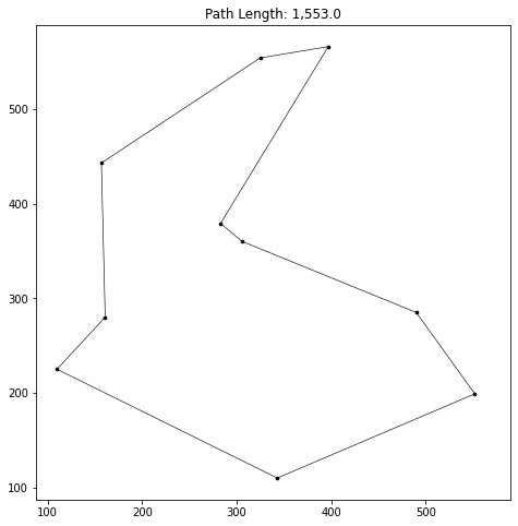
It’s interesting to compare this path to a greedy path achieved by starting from a random node and selecting the nearest next node until we’ve been through all nodes.
greedy_path = ants.greedy()
ants.plot_path(greedy_path)
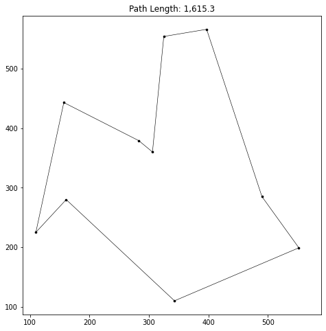
We see that the path is longer than the one found by the ants.
100 nodes
ants = AntOpt(points100, n_ants=20)
ants
Optimizing with 100 cities, n_iter=300, n_ants=20, alpha=2, beta=3, rho=0.85, Q=0.3
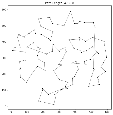
best_path = ants.run_ants()
ants.plot_path(best_path)
40%|███▉ | 119/300 [02:50<04:19, 1.43s/it] breaking at iteration: 119 with best path length: 4736.8152396678925
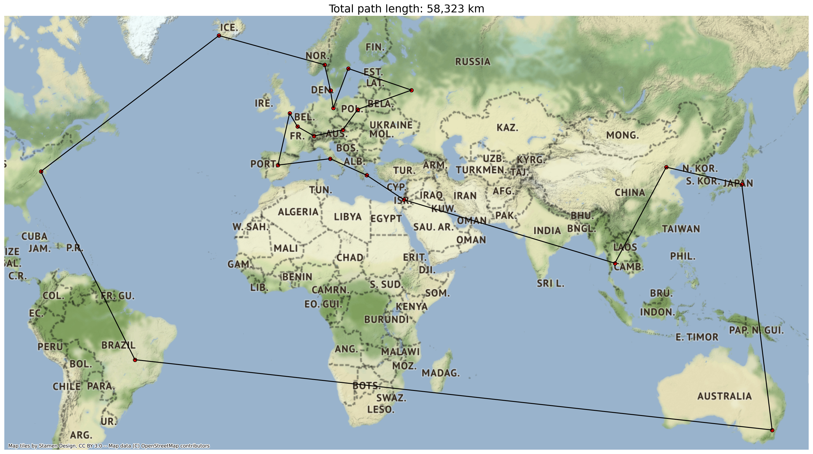
Actual cities example
In this example I’ll use capital cities around the world, and find a path using the ants optimization.
# imports and setting up

import geopandas as gpd
import contextily as ctx

capitals = pd.read_csv('data/capitals.csv', usecols=['CountryName','CapitalName', 'CapitalLatitude', 'CapitalLongitude', 'ContinentName'])  # from https://www.kaggle.com/nikitagrec/world-capitals-gps

# filter to specific countries
countries = ['United Kingdom', 'France', 'Italy','Spain','Germany','Sweden','Norway','Denmark','Iceland','Greece','Switzerland','Austria','Poland','Russia','Israel','United States','Australia','Japan','Brazil','China','Thailand']

capitals = capitals[capitals['CountryName'].isin(countries)].copy()

capitals.dropna(subset=['CapitalName'], inplace=True)

# Get capital lat/lon as points
capitals_points = capitals[['CapitalLongitude','CapitalLatitude']].values

# Convert to GeoPandas Dataframe
gdf_capitals = gpd.GeoDataFrame(capitals, geometry=gpd.points_from_xy(capitals.CapitalLongitude, capitals.CapitalLatitude))
gdf_capitals.crs = 'epsg:4326'

fig, ax = plt.subplots(figsize=(24,24))
gdf_capitals.to_crs('epsg:3857').plot(ax=ax, color='r', edgecolor='k')
ctx.add_basemap(ax)
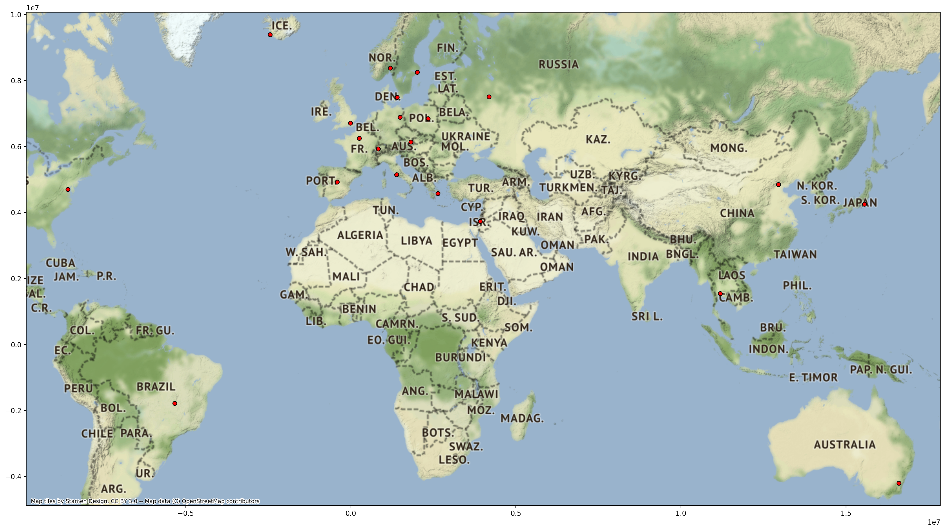
Next we optimise a path through the cities:
ants = AntOpt(capitals_points, dist='geo', n_iter=200, n_ants=15, rho=0.85)

best_path = ants.run_ants()

# connect points to create path as a geodataframe
worldpath = LineString(gdf_capitals.iloc[best_path]['geometry'].values)
gdf_path = gpd.GeoDataFrame(geometry=[worldpath], crs='epsg:4326')

# plot path
fig, ax = plt.subplots(figsize=(24,24))
gdf_capitals.to_crs('epsg:3857').plot(ax=ax, color='r', edgecolor='k')
gdf_path.to_crs('epsg:3857').plot(ax=ax, color='black')
ctx.add_basemap(ax)
ax.set_axis_off()
ax.set_title(f'Total path length: {path_length:,.0f} km', fontsize=18)
The ant optimization algorithm can be extended to other variations of the TSP, e.g. capacity constrained vehicle routing, where the vehicles have a limited capacity of goods they need to deliver to the cities. The only change to the ant optimization algorithm would be to limit the possible transition nodes an ant can choose and keep track of the capacity each ant carries.