Stocks
The stock market is known to be a highly complex and unpredictable dynamic system, driven by multiple inputs on multiple time scales. It has even been theorised (Efficient Market Hypothesis) that one cannot beat the stock market, as it is highly efficient and always reflects all existing information in the market.
At the end of the day the stock market is a kind of an auction where people sell shares to people willing to buy shares in a given company, creating a balance which is reflected in the current share price of the company. It is in general thought that the stock market reflects the overall economy as when the economy is growing people will have money to invest creating a bull market, whereas when the economy is in decline people will sell creating a bear market.
The economy as a whole is really composed of multiple somewhat independent parts as reflected in the past year, where an event such as a pandemic although at first hitting everyone at once causing a big collapse around March, quickly saw the stock prices of particularly the tech company rising sharply to rates even higher than those before the pandemic.
Overall investing in stocks especially these days is a good investment for significant returns as compared to any saving accounts or risk-free investments. Especially taken inflation into account, free-standing money actually loses value, it is therefore a wise decision to have it invested somewhere, and as long as its not all of ones earnings (as there is always risk) it can pay off.
For a casual investor like my self, who’s started only recently (Around August) to invest some money, the relevant time scales range from days through weeks and months to years. I am not interested be constantly checking the stock values at an hourly or sub-hourly frequency. I see it more as a mid to long-range investment believing in the overall trend of particular markets.
People have come up with various indicators to guide the investor on when might be a good time to buy or sell, which I’ve used below. There is no forecasting involved and no price predictions, these are simply indicators of market movement, which in some cases may seem quite arbitrary, but the idea is that by combining a number of these indicators a useful signal may come through with potential for profit. Although individual agents within the market are highly unpredictable, overall there are some patterns or behaviours of the market as a whole which are recurring and have been demonstrated to be good to take note of.
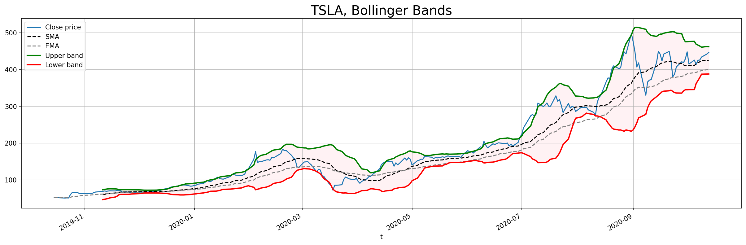
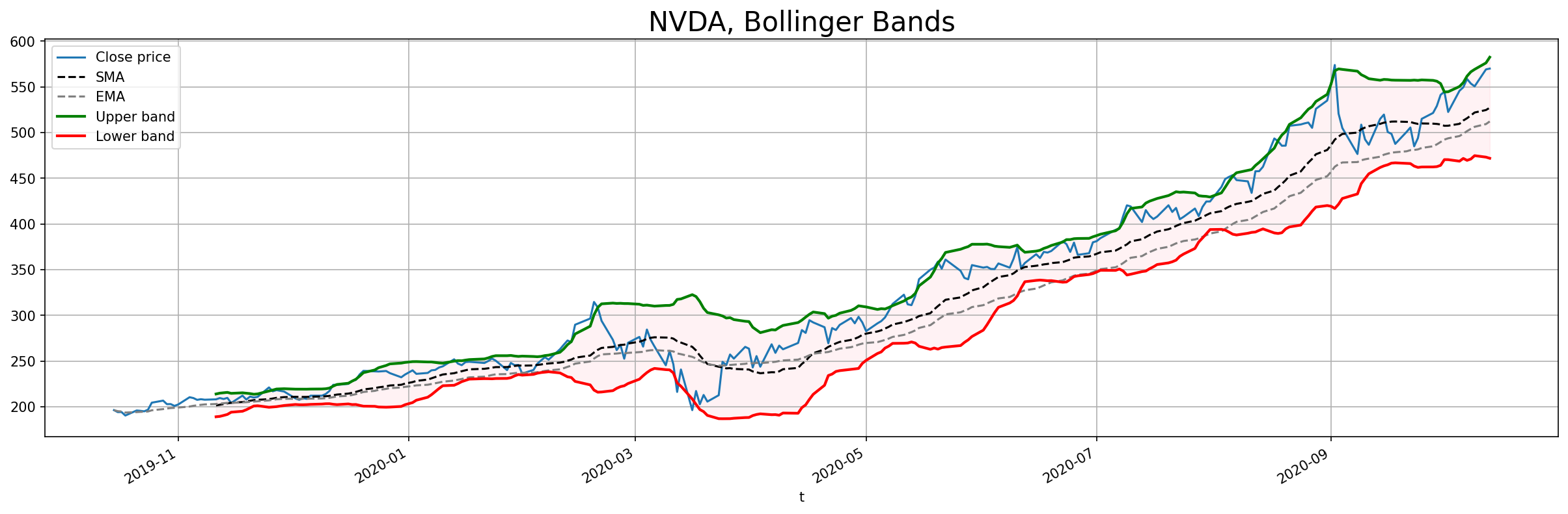
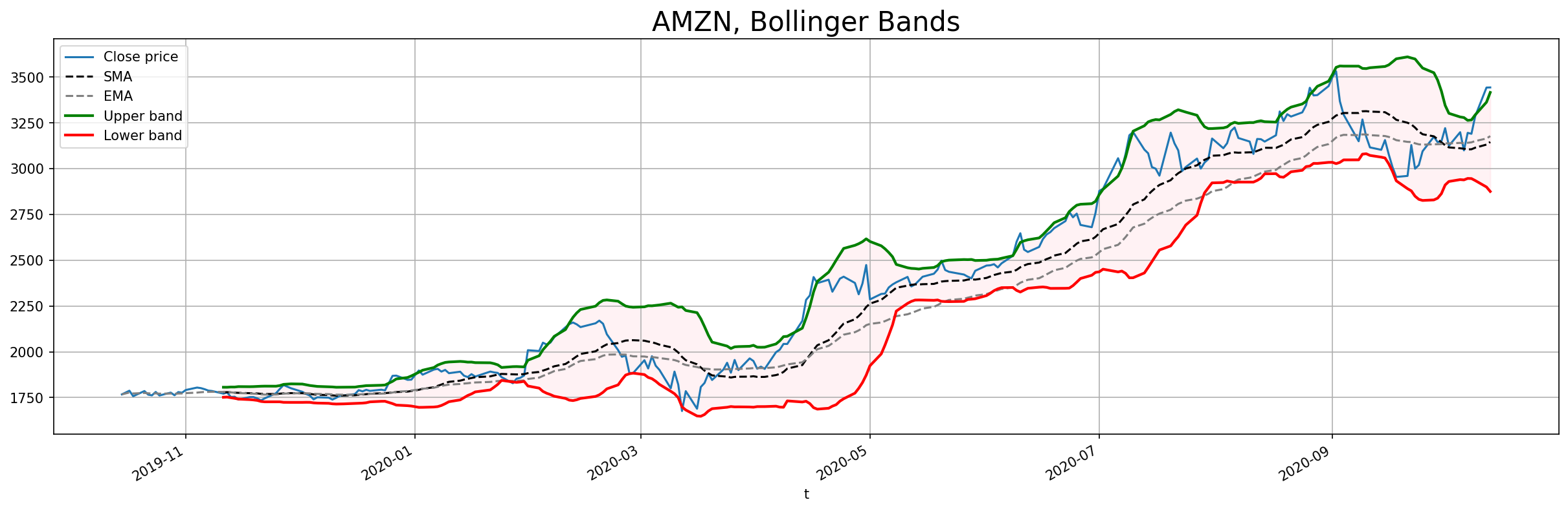
Bollinger Bands
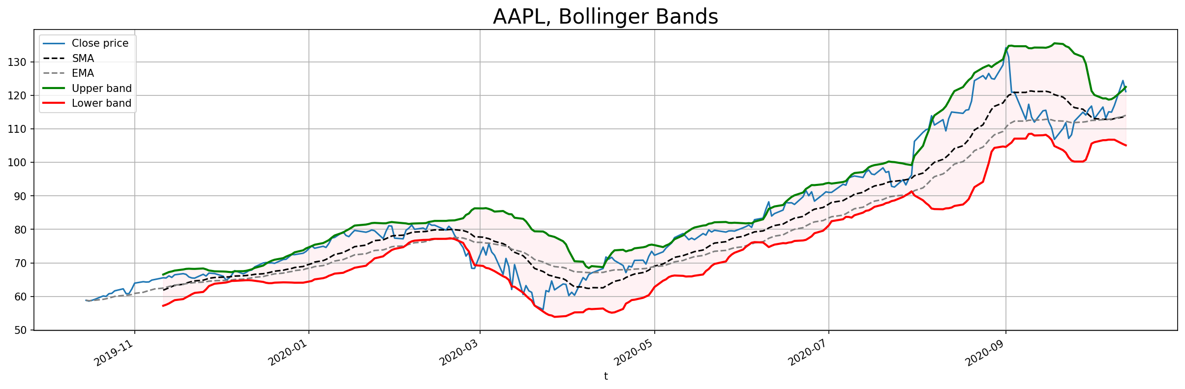
The Bollinger bands represents two bands above and below the close price of a stock. The bands are obtained as $n$ standard deviations of the moving average of the closing price with window $w$ above and below the moving average.
\[{\rm bands} = {\rm SMA}_w({\rm close}) \pm n \sigma({\rm close}),\]where $SMA_w$ is the simple moving average with period $w$ and $\sigma$ is the standard deviation. close is the time series of the stock closing price.
Typical values are $w=20, n=2$.
The idea is that these two bands represent bounds within which the stock is trading and when the stock reaches the top band it is a sign that the stock is being over bought and is likely that a down trend will start, and vice versa for the lower band.
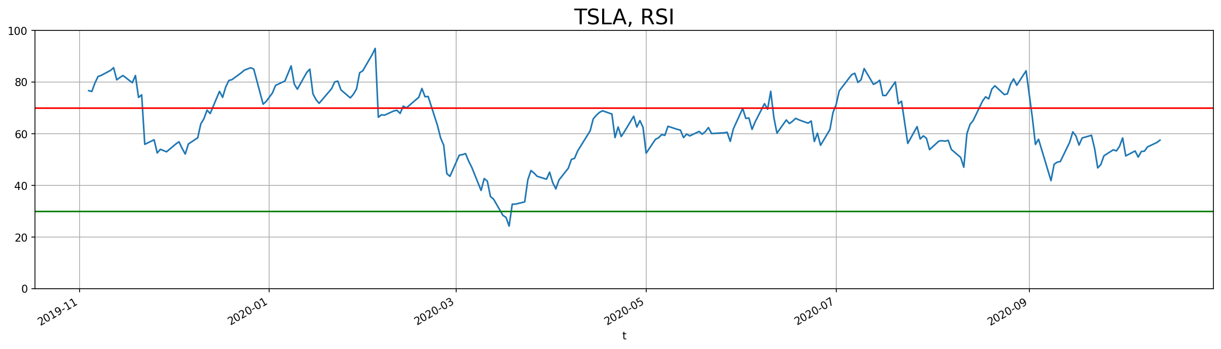
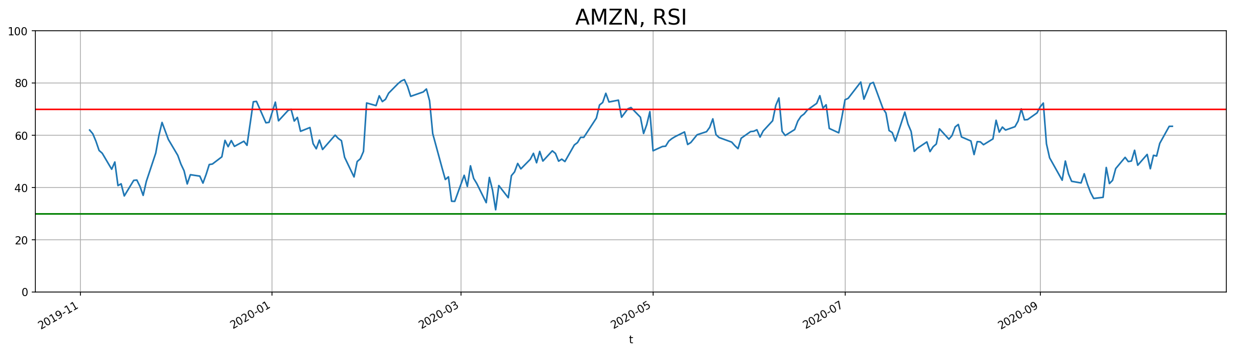
Relative Strength Index (RSI)
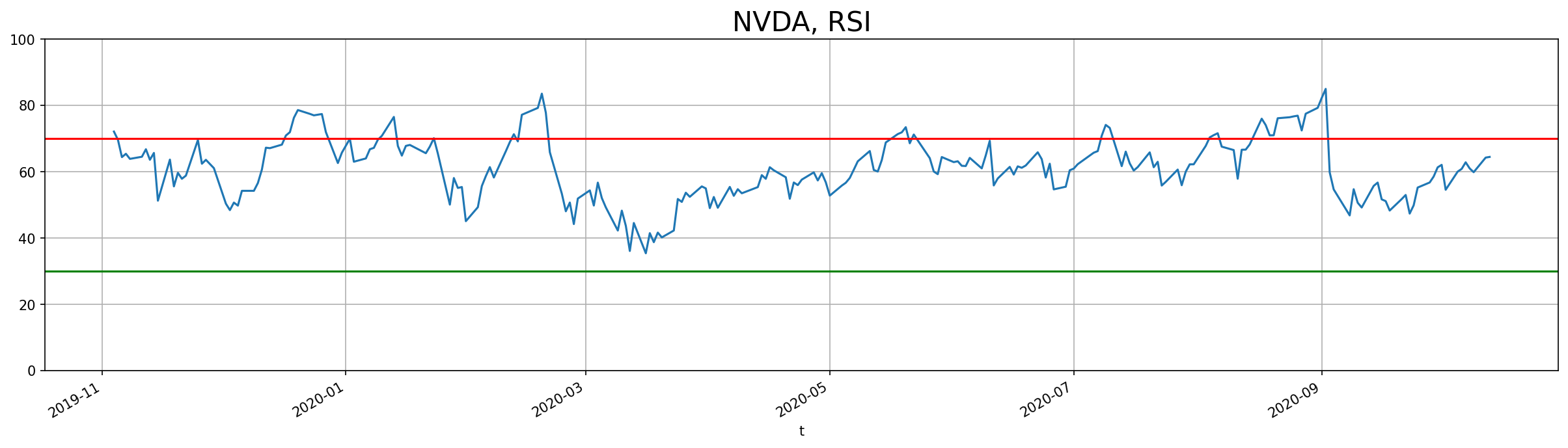
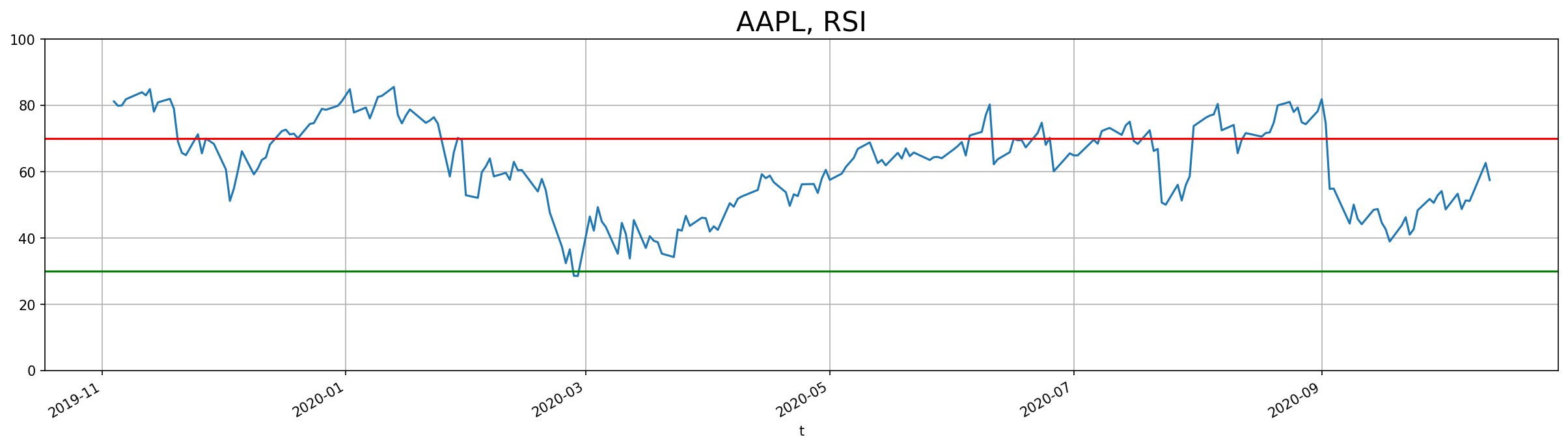
The RSI is a value between 0 to 100 which is obtained from the ratio of the exponentially moving averages of the gains and loses in a given period. Where a gain or loss is the difference between consecutive closing prices, gain if positive, loss if negative, however the absolute value is used. The ratio is finally scaled between 0 and 100. The RSI values of 30 and 70 are considered the bounds which indicate over bought and over sold stocks and at which point a momentum shift is anticipated.
\[{\rm RSI} = 100\left(1- \frac{1}{1 + \frac{ {\rm EMA}(N,\ {\rm gains})}{ {\rm EMA}(N,\ {\rm losses})}}\right),\]where $1/(1+N) = \alpha$ is the smoothing coefficient, which determines how much to weigh the current value and the previous values and is typically chosen to be $N=14$, for the exponential moving average (EMA) which is defined recursively for a series $y_1$, as $V_i = \alpha V_{i-1} + (1-\alpha)y_i$, with $V_1 = y_1$, with $V_i$ being the value of the EMA.
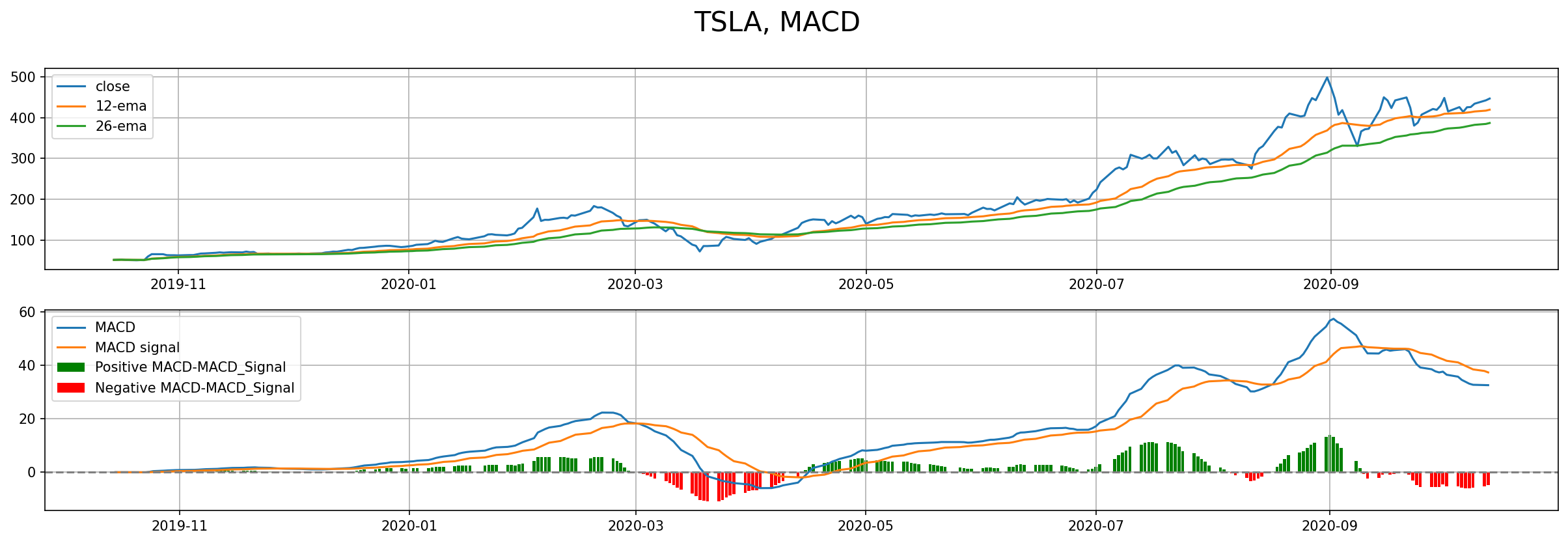
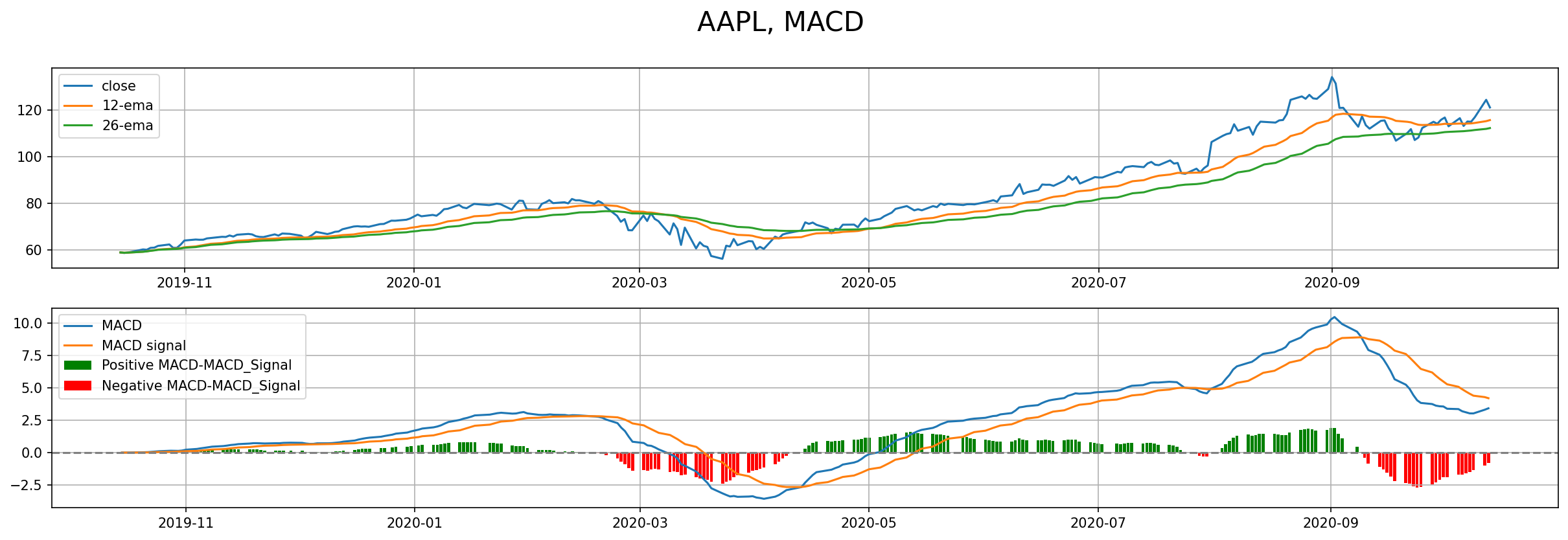
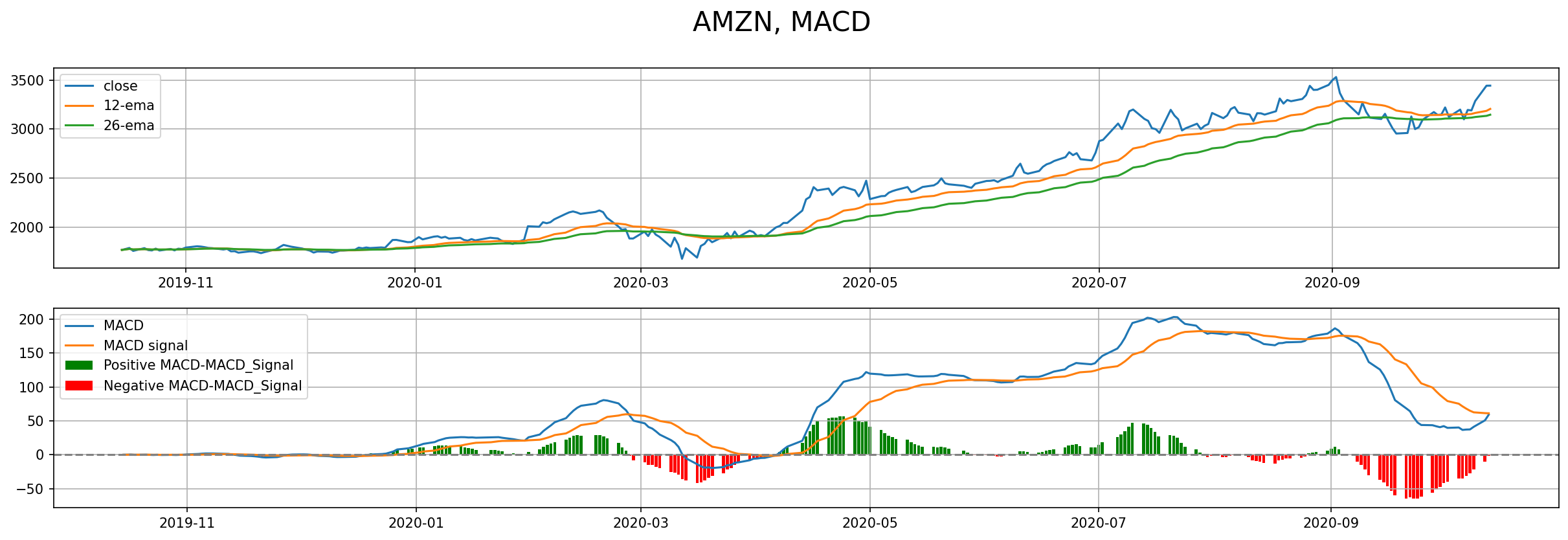
MACD (Moving Average Convergence Divergence)
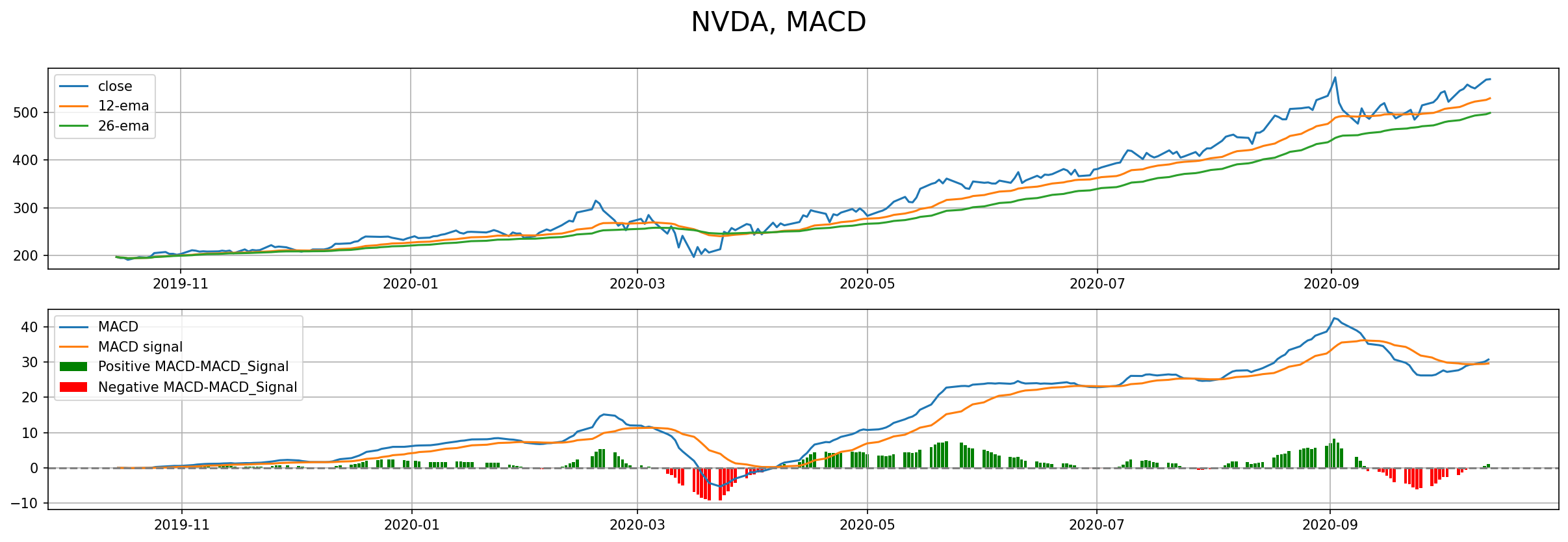
The MACD compares the trends over a short (12 periods) and long (26 periods) periods using the exponentially weighted average. The MACD is then the difference between the short and long term trends. The MACD goes further to calculate the 9 period EMA of the MACD, called the MACD signal and finally compares the two. The being is that when the signal trend crosses the MACD trend there is a momentum shift in the market in the direction dictated by the direction of crossing. The difference between the two then also indicates the strength of this momentum.
\[{\rm MACD} = EMA(12, {\rm close}) - EMA(26, {\rm close}), \\ {\rm MACD}_{signal} = {\rm EMA}(9, {\rm MACD}).\]Code
Below I’ve implemented the above indicators in Python and used them for a number of stocks using the Finnhub API.
The python class for dealing with the stocks data:
class Stock():
    def __init__(self, symbol: str, start: dt.datetime = None, end: dt.datetime = None):
        self.symbol = symbol
        self.api_key = api_key
        if end is None:
            self.end = int(dt.datetime.now().replace(microsecond=0).timestamp())
        else:
            self.end = end

        if start is None:
            # year start
            self.start = int((dt.datetime.now() - dt.timedelta(days=365)).timestamp())
        else:
            self.start = start

        self.candles = self._get_candles()

    def _get_candles(self):
        url = f'https://finnhub.io/api/v1/stock/candle?symbol={self.symbol}&resolution=D&from={self.start}&to={self.end}&token={self.api_key}'

        res = requests.get(url)
        if res.status_code != 200:
            print(f"Bad request status {res.status_code}")
            print(res.text)
            return

        candles = pd.DataFrame(res.json())
        candles['t'] = pd.to_datetime(candles['t'], unit='s')
        candles = candles.set_index('t')
        print(f"last available date: {candles.index[-1].date()}")
        return candles[['o','c','h','l']]

    def RSI(self):
        candles_rsi = self.candles.copy()
        candles_rsi.loc[:, 'gain'] = (candles_rsi['c'] - candles_rsi.shift(1)['c'])
        candles_rsi['U'] = candles_rsi['gain'].apply(lambda x: x*(x>0))
        candles_rsi['D'] = candles_rsi['gain'].apply(lambda x: np.abs(x*(x<0)))
        candles_rsi['RS'] = (candles_rsi['U'].ewm(alpha=1/14, min_periods=14).mean()
                            / candles_rsi['D'].ewm(alpha=1/14, min_periods=14).mean())
        candles_rsi['RSI'] = 100 - 100/(1 + candles_rsi['RS'])

        fig,ax = plt.subplots(figsize=(20,5))
        candles_rsi['RSI'].plot(ax=ax)
        ax.axhline(y=70, color='red')
        ax.axhline(y=30, color='green')
        ax.set_ylim(0,100)
        plt.grid()
        plt.title(f"{self.symbol}, RSI", fontsize=20)
        return candles_rsi

    def bollinger_bands(self, periods:int = 20, std:int = 2):
        candles_bol = self.candles.copy()

        sma = candles_bol['c'].rolling(periods, min_periods=periods).mean()
        ema = candles_bol['c'].ewm(periods).mean()
        sig = candles_bol['c'].rolling(periods).std()
        upper2 = sma + 2*sig
        lower2 = sma - 2*sig

        fig,ax=plt.subplots(figsize=(20,6))
        candles_bol.plot(y='c', ax=ax, label='Close price')
        sma.plot(color='black', linestyle='--', ax=ax, label='SMA')
        ema.plot(color='gray', linestyle='--', ax=ax, label='EMA')
        upper2.plot(color='g', linestyle='-', ax=ax, linewidth=2, label='Upper band 2')
        lower2.plot(color='r', linestyle='-', ax=ax, linewidth=2, label='Lower band 2')
        plt.fill_between(lower2.index, lower2, upper2, alpha=0.2, color='pink')
        plt.legend()
        plt.grid()
        plt.title(f"{self.symbol}, Bollinger Bands", fontsize=20)
        return

    def MACD(self):
        """
        Moving Average Convergence Divergence
        """
        candles_macd = self.candles.copy()
        long_ema = candles_macd['c'].ewm(26).mean()
        short_ema = candles_macd['c'].ewm(12).mean()
        macd = short_ema - long_ema
        macd_signal = macd.ewm(9).mean()
        macd_diff = macd - macd_signal

        fig,ax=plt.subplots(2, 1, figsize=(20,6))
        ax[0].plot(candles_macd.index, candles_macd['c'], label='close')
        ax[0].plot(short_ema.index, short_ema, label='12-ema')
        ax[0].plot(long_ema.index, long_ema, label='26-ema')

        ax[1].plot(macd.index, macd, label='MACD')
        ax[1].plot(macd_signal.index, macd_signal, label='MACD signal')
        pos_macd_diff = macd_diff[macd_diff>=0]
        neg_macd_diff = macd_diff[macd_diff<0]
        ax[1].bar(pos_macd_diff.index, pos_macd_diff, color='green', label='Positive MACD-MACD_Signal')
        ax[1].bar(neg_macd_diff.index, neg_macd_diff, color='red', label='Negative MACD-MACD_Signal')
        ax[1].axhline(color='gray', linestyle='--')
        ax[0].legend()
        ax[1].legend()
        plt.grid()
        fig.suptitle(f"{self.symbol}, MACD", fontsize=20)
        return

    def sharpe_ratio(self):
        """
        Calculate sharpe ratio assuming 0 return for risk-free
        """
        df = self.candles.copy()
        df['daily_return'] = df['c'].pct_change()
        df['cumulative_return'] = df['daily_return'].cumsum()
        avg_return = df['daily_return'].mean()
        std_return = df['daily_return'].std()
        print(f"Cumulative return: {df['cumulative_return'].iloc[-1]*100:.2f}%")
        print(f"Sharpe Ratio: {avg_return/std_return:.2f}, from: {df['daily_return'].index[0].date()}")
        fig, ax = plt.subplots(figsize=(16, 4))
        ax.plot(df.index, df.cumulative_return, label='cumulative return')
        ax.legend()
Examples:
To get the stock closing prices (1 year default):
tsla = Stock('TSLA')
apple = Stock('AAPL')
nvidia = Stock('NVDA')
amazon = Stock('AMZN')
To obtain the indicators we use:
tsla.bollinger_bands()
tsla.RSI()
tsla.MACD()
Outputs:
Tesla
Nvidia
Apple
Amazon
Portfolio optimization
The main question of investing is how to allocate an existing budget across a number of assets (equity, commodities, bonds). Given a set of allocated weights $w_i$: $R_p = \sum_i w_i R_i$, where $R_i$ is the return of asset $i$.
The expected return of the portfolio is then given by: \(E(R_p) = \sum_{i} w_i E(R_i).\)
The main realization of Markovitz the father of modern portfolio theory was that the risk in a given portfolio is given by the variance of the portfolio’s returns, which in turn is captured by covariance matrix of the assets’ returns, which includes both the variance of the individual assets and their correlations, which is the main insight leading the wisdom that a good portfolio meaning having the best return for a given level of risk needs to be diversified in such away that the assets are not correlated to each other.
To see how the covariance comes out, I derive the variance of the portfolio’s return:
\[V(R_p) = E(R_p^2) - E^2(R_p) = \\ E\left[\sum_{i,j}w_iw_jR_iR_j\right] - \sum_{i,j}E(R_i)E(R_j) = \\ \sum_{i,j}(w_iw_j)\left[E(R_iR_j) - E(R_i)E(R_j)\right]\]The term in the square brackets is by definition the covariance of assets $i$ and $j$, the variance of the portfolio returns is therefore given by:
\[\begin{align} V(R_p) = {\bf w}^T \Sigma {\bf w}, \end{align}\]where $\Sigma$ is the covariance matrix of the assets’ returns.
One of the popular portfolio selection or optimization techniques is the Risk Parity portfolio where the idea is to allocate weights to achieve equal risk contribution from each asset to the overall portfolio risk or volatility. This has been found to overcome issues with the mean-variance and minimum variance approaches which tend to concentrate most of the weight on few assets.
The portfolio volatity from (1) can be written as teh sum of the risk contributions of each asset using Euler’s Homogenous Function Theorem and the fact that $V(w)$ is homogeneous of order 1 in $w$,
\[V(w) = \sum_i w_i\frac{\partial V({\bf w})}{\partial w_i} = \sum_i w_i \frac{ \Sigma {\bf w}}{V(w)} = \sum_i v_i\]Where $v_i$, the term inside the sum is the contribution of asset $i$ to the overall volatility. In general if we want each asset to contribute $b_i$ to the total portfolio risk, with $\sum b_i = 1$, e get the condition for the risk parity portfolio $v_i(w) = b_iV(w)$, for equal risk contribution $b_i = \frac{1}{N}$.
\[w_i (\Sigma {\bf w})_i = ({\bf w}^T \Sigma {\bf w}) b_i.\]The optimization problem can then be forumlated as minimizing the sum of squared errors between the desired risk contribution and the actual:
\[J({\bf w}) = \sum_i \left[w_i (\Sigma {\bf w})_i - ({\bf w}^T \Sigma {\bf w})b_i \right]^2,\] \[w = \argmin_w J({\bf w}) \quad \mid \quad w_i \ge 0\]