Transformers

Since the seminal paper on transformers “Attention is All You Need”, transformers have revolutionized deep learning and have become the most popular architecture, applied to a variety of different problems and modalities. In text for tasks such as: text generation (e.g. GPT-3), translation (BERT), classification, in vision with image classification (ViT), object detection and text-to-image generation as well as audio with transcription (Whisper).

The transformer architecture is a highly expressive, efficient and parallelizable way of processing information on a set. The high expressiveness, which gives it the ability to learn interesting and generalizable relationships in the training data, originates from the attention mechanism, which allows any element in the set to have attention to other elements in the set, giving each element additional context, which may be useful for the given task. Architectures such as RNN and CNN were designed precisely to take advantage of data structure in sequences and images, i.e. the sequential nature of RNN and the spatial equivariant nature of the convolutional layers (translation of the input results in a translated output) as well as the spatial inductive bias (the convolution filter identify local features), but these inductive biases are exactly what limits their abilities as compared to transformers. In the case of RNN/LSTM, information is processed sequentially (e.g. a sentence), such that in order for a given word to process information from a work far in the beginning of th text, a significant amount of training data may be required, as the signal gradient signals weakens deeper in the network. Similarly in CNNs, the global nature of the transformer allows it to take advantage of the whole image as opposed to only use local features.

How Transformers work

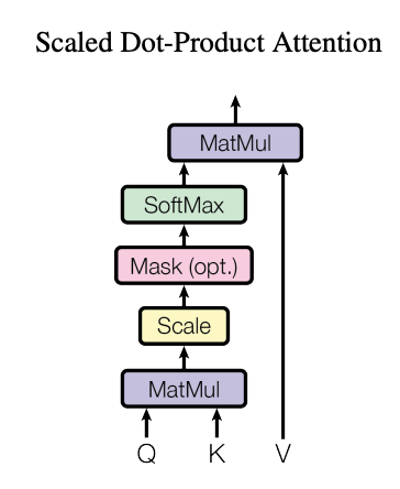
The scaled Dot-Product Attention diagram from “Attention is all you need” paper

The way the transformer achieves this expressive information processing on a set is simple but powerful. Since the set doesn’t have necessarily a notion of a vicinity of an element to another, unlike a time series for example, each element (assuming is already represented as a numerical vector) is first project to the space of queries, keys and values, with learnable weights, then the attention that each element has for every other element depends on the vicinity of the query to the key, with the vicinity defined by a simple dot product, normalizing those dot products using a softmax and calculating a weighted sum with the values, we get a new representation for each element as a combination of the values of all the elements weighted by the relevant attention. Those projection weights will be learned using back-propagation and stochastic gradient descent to solve a specific task.

Given a set of $T$ queries, keys and values of dimensions $d_k, d_k$ and $d_v$, respectively.

The attention vectors are then given by:

\[Attention =(Q,K,V) = {\rm softmax} \left(\frac{QK^T}{\sqrt{d_k}}\right) V,\]

where the softmax is applied on the last dimension to normalize the attention weights to apply to each element’s values vector. The additional factor of $\sqrt{d_k}$ is an important detail which normalizes the values of the query, key product in order to avoid saturating the softmax, as we are summing $d_k$ values in each row.

$Q K^T$ gives a matrix of size $T \times T$, and the final attention gives a matrix of size $T\times d_v$. This generalizes to batched sequences by simply adding an additional dimension at the beginning of the batch size.

In PyTorch the dot-production attention can be implemented as:

from typing import Tuple
import torch
from einops import einsum
import torch.nn.functional as F
import math

def scaled_dot_prod(q: torch.Tensor, k: torch.Tensor , v: torch.Tensor) -> Tuple[torch.Tensor, torch.Tensor]:

  d_k = q.shape[-1]

  # b - batch size, n - sequence length
  qk_scores = einsum(q, k, "b s i j, b n k j -> i k") / math.sqrt(d_k)

  # normalize with softmax
  attn_weights = F.softmax(attn_logits, dim=-1)

  # multiply by values
  values = torch.matmul(attn_weights, v)

  return values, attn_weights

The authors then extend the idea of the attention single attention mechanism to multiple ones with multi-head attention:

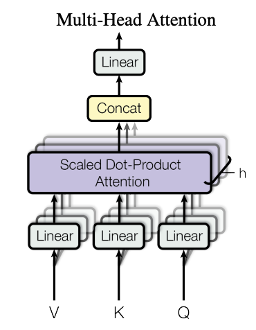
The Multi-Head Attention diagram from “Attention is all you need” paper

The motivation here is that whereas a single attention allows each element to attend with varying weights to any other element, it is still limited to only a single context for each element, but it may be the case the there might be other useful contexts to learn for each element, and this is achieved by having multiple heads $h$. The input to the model is typically a sequence of elements (tokens in the case of text), each with an embedding of dimension $d_{model}$, to bring the elements to the space of queries, keys and values we use the projection matrices $W^Q_{1..h},\ W^K_{1..h},\ W^V_{1..h}$, i.e. one triplet of q,k,v matrices per head. The dimensions of these projection matrices are given by $d_{model}\times d_k$ with $d_k,d_v = d_{model}/h$, such that after the attention outputs from each head are concatenated, we get a vector of size $T\times d_{model}$, which is finally projected one more time with $W^O \in {\mathbb R}^{d_{model} \times d_{model}}$.

In a more compact notation these steps can be written as in the paper:

\[{\rm MultiHead}(Q, K, V) = {\rm Concat}(head_1, ..., head_h)W^O; \\ head_i = {\rm Attention}(QW^Q_i, KW^K_i, VW^V_i).\]

In PyTorch:

import torch
import torch.nn as nn
from einops import rearrange


class MultiheadAttention(nn.Module):
  def __init__(self, input_dim: int, model_dim: int, n_head: int):
    super().__init__()

    self.model_dim = model_dim
    self.n_head = n_head
    d_k = model_dim // n_head

    # combine the 3 projection matrices and heads into a single projection
    # for efficiency, as it's faster to make a single matrix multiplication
    # rather than 3 separate ones
    self.qkv_proj = nn.Linear(input_dim, 3*model_dim)
    self.o_proj = nn.Linear(model_dim, model_dim)

  def forward(self, x: torch.Tensor):

    # project input into q,k,v space
    qkv = self.qkv_proj(x)

    # separate into q, k, v
    qkv = rearrange(qkv, "b n (h d) -> b h n d", h=self.n_head)

    q, k, v = qkv.chunk(3, dim=-1)

    values, attention = scaled_dot_prod(q, k, v)

    # concatenate heads
    values = rearrange(values, "b h n d -> b n (h d)")

    # final projection
    o = self.o_proj(values)

    return o

Example:

multi_head = MultiheadAttention(input_dim=4, model_dim=8, n_head=2)

x = torch.randn(3, 3, 4) # batch 3, seq len 2, embedding dim 4
out = multi_head(x)

# >
# qkv shape after projection: torch.Size([3, 3, 24])
# qkv shape after rearrangement: torch.Size([3, 2, 3, 12])
# q shape after chunking: torch.Size([3, 2, 3, 4])
# values shape after attention dot product: torch.Size([3, 2, 3, 4])
# values shape after concatenation of all heads: torch.Size([3, 3, 8])
# Final output shape : torch.Size([3, 3, 8])