Machine Learning classification
The purpose of this article is to serve as a playground for demonstrating the use of some of the common supervised classification algorithms using the scikit-learn library, which is a widely used popular machine learning library with a very detailed documentation and plenty of examples.
We start by generating data with labels using the built-in function in scikit-learn called make_moons to create a moon shaped data set with two features (x and y coordinates) separated in to two classes with some added noise. as shown below.
%matplotlib inline
import sklearn.datasets
import matplotlib.pyplot as plt
import matplotlib
import numpy as np

matplotlib.style.use('ggplot') #makes plots look pretty

# Generate a dataset and plot it
np.random.seed(0)
X, y = sklearn.datasets.make_moons(200, noise=0.2)
plt.scatter(X[:,0], X[:,1], s=40, c=y, cmap=plt.cm.Spectral)
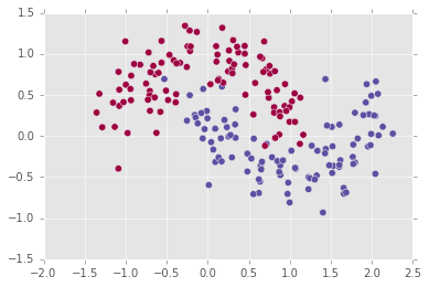
The task of a classifier trained on this data set is to provide a decision boundary which will separate the two classes in a generalizable way, such that future test points, unseen by the classifier and which are taken from the same distribution, will be correctly classified.
For visualization purposes we have the following function which plots the decision boundary,
def plot_decision_boundary(model,X,y):
    padding=0.15
    res=0.01

    #max and min values of x and y of the dataset
    x_min,x_max=X[:,0].min(), X[:,0].max()
    y_min,y_max=X[:,1].min(), X[:,1].max()

    #range of x's and y's
    x_range=x_max-x_min
    y_range=y_max-y_min

    #add padding to the ranges
    x_min -= x_range * padding
    y_min -= y_range * padding
    x_max += x_range * padding
    y_max += y_range * padding

    #create a meshgrid of points with the above ranges
    xx,yy=np.meshgrid(np.arange(x_min,x_max,res),np.arange(y_min,y_max,res))

    #use model to predict class at each point on the grid
    #ravel turns the 2d arrays into vectors
    #c_ concatenates the vectors to create one long vector on which to perform prediction
    #finally the vector of prediction is reshaped to the original data shape.
    Z = model.predict(np.c_[xx.ravel(), yy.ravel()])
    Z = Z.reshape(xx.shape)

    #plot the contours on the grid
    plt.figure(figsize=(8,6))
    cs = plt.contourf(xx, yy, Z, cmap=plt.cm.Spectral)

    #plot the original data and labels
    plt.scatter(X[:,0], X[:,1], s=35, c=y, cmap=plt.cm.Spectral)
Logistic Regression
The first algorithm is logistic regression, which despite the name is a classification algorithm and not a regression algorithm. Logistic regression is a linear classifier which uses the sigmoid function with trained weights and bias to assign a probability for a given data point.
\[\sigma(x; W,b)=\frac{1}{1+e^{-(W x+b)}}\]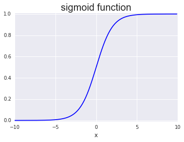
Using scikit-learn we train a logistic regression classifier and plot its decision boundary
from sklearn.linear_model import LogisticRegression
model = LogisticRegression()
model.fit(X, y)
plot_decision_boundary(model,X,y)
the fitting model parameters:
LogisticRegression(C=1.0, class_weight=None, dual=False, fit_intercept=True,
          intercept_scaling=1, max_iter=100, multi_class='ovr', n_jobs=1,
          penalty='l2', random_state=None, solver='liblinear', tol=0.0001,
          verbose=0, warm_start=False)
Some hyper parameters of interest: penalty=’l2’ sets the cost function type to be the square of the error as opposed to ‘l1’ which is the absolute
value. The parameter C=1.0 controls (inversely) the regularization which is responsible for preventing over-fitting of the trained weights. Small values correspond to stronger regularization.
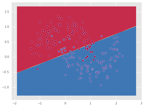
We see that the linear classifier found the best linear separation it could find, which however is not good since the particular dataset is not linearly separable.
SVM - Support vector machine
The next algorithm is the support vector machine (svm) algorithm. SVM is also a linear classifier which tries to find the boundary by focusing on the two closest points from different classes (support vectors) and finds the line that is equidistant to these two points as the separation boundary. SVMs however have the kernel option which allows to represent the data in higher dimensions. This allows to separate data that are not separable linearly in the original space, but are linearly separable in a higher dimensional space.
from sklearn.svm import SVC
model = SVC(kernel='linear')
print model.fit(X, y)
plot_decision_boundary(model,X,y)
The model training parameters:
SVC(C=1.0, cache_size=200, class_weight=None, coef0=0.0,
  decision_function_shape=None, degree=3, gamma='auto', kernel='linear',
  max_iter=-1, probability=False, random_state=None, shrinking=True,
  tol=0.001, verbose=False)
Below we show the resulting boundary for a ‘linear’ and ‘rbf’ kernels.
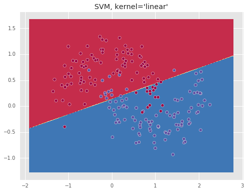
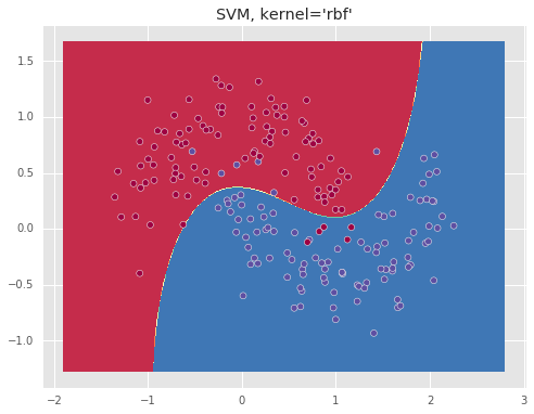
The ‘rbf’ kernel which essentially represents the data in an infinite dimensional space, allows to separate the data well.
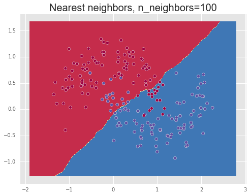
Nearest neighbors
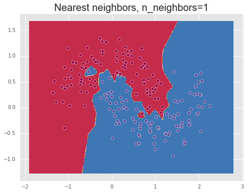
The next algorithm is the nearest neighbors algorithm, considered the most basic machine learning algorithm due to the simplicity of the idea, which is that the class of a given test point is determined by a majority vote of its \(n\) nearest neighboring points.
from sklearn.neighbors import KNeighborsClassifier
model = KNeighborsClassifier(n_neighbors=5)
model.fit(X, y)
plot_decision_boundary(model,X,y)
The model training parameters:
KNeighborsClassifier(algorithm='auto', leaf_size=30, metric='minkowski',
           metric_params=None, n_jobs=1, n_neighbors=10, p=2,
           weights='uniform')
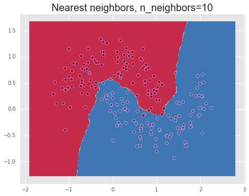
We show the results of using different values for the number of neighbors, n_neighbors=1,10,100, demonstrating over-fitting or high variance for a small number of neighbors, meaning that the model captures too much of the noise in the data and thus will note generalize well to unseen data points, and under-fitting or a high bias for a large number of neighbors. Finally, a value between these two extremes, such as 10, manages to separate the data relatively well.
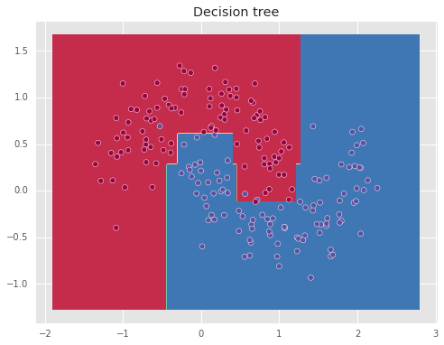
Decision tree
The next algorithm is the decision tree, which uses intersecting vertical lines to create the decision boundary, allowing to obtain non-linear decision boundaries.
from sklearn.neighbors import KNeighborsClassifier
from sklearn import tree
model = tree.DecisionTreeClassifier(min_samples_leaf=3)
model.fit(X,y)
plot_decision_boundary(model,X,y)
DecisionTreeClassifier(class_weight=None, criterion='entropy', max_depth=None,
            max_features=None, max_leaf_nodes=None, min_samples_leaf=3,
            min_samples_split=3, min_weight_fraction_leaf=0.0,
            presort=False, random_state=None, splitter='best')
Here the parameter min_samples_leaf controls the minimum number of samples required to be in a leaf, which helps to prevent over-fitting.