Neural Networks
The human brain is arguably the most sophisticated and complicated device ever “created”. The thought of humans trying and succeeding to some extent, to understand the way the brain works is astonishing. The pursuit of understanding the human brain has naturally led to the formation of the field of artificial intelligence, in which people are trying to produce an intelligent entity capable of reasoning and understanding the world just as we do or even better.
Humans have created math as a way to abstract nature and make it comprehensible to their own brains. As Einstein famously pointed out, it is remarkable that mathematics, being a product of human thought, is capable of describing nature and reality so well.
The human brain is composed of billions of interconnected neurons - brain cells, forming the neural network of the brain. The neurons communicate with each other though electrical pulses, governed by known chemical and physical laws, governing the brain, and that’s it, there is no extra magic, this seemingly basic framework, is capable of making us intelligent, being able to learn, think, and create. In trying to create a machine that can learn in a similar way, a good starting point would be to see what the brain does and try to imitate it. A single neuron cell has a body which governs the activity of the cell, Dendrites which receive signals from other neurons, and Axons which transmit signals to other neurons through junctions called synapses.
Artificial neuron
A simple abstraction of the biological neuron, would be a computational unit which receives some input from multiple sources, sums the inputs with some specific weights for each input, and perhaps an overall bias as well. This summation then goes through some activation function which determines the output of the neuron based on its input, which serves as the input for other neurons.
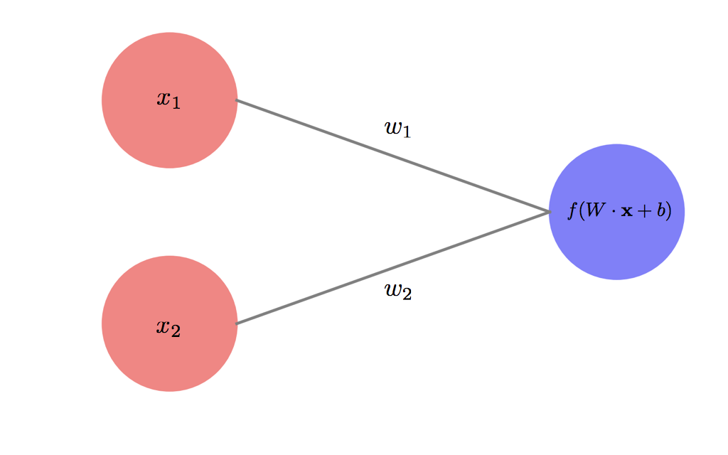
We can imagine multiple layers of such artificial neurons interconnected,with the activation of one layer of neurons influencing the activation of the next, forming an artificial neural network. Remarkably, using a non-linear activation function makes such a deep (more than two layers) neural network a “universal function approximater”, i.e. it can approximate any function from the inputs to the output by appropriately tuning its weights.
Learning
The question is then, how does a neural network learn? At this point this question becomes a problem in optimization. A network’s output for a given input is uniquely determined by its set of weights and biases, forming a multidimensional space with the different parameters as its axis. Given the desired output of the network, we have some loss or cost function which determines how far is the network from outputting the desired value. Therefore the task of learning is reduced to the task of minimizing this loss function through modifying the weights and biases connecting the artificial neurons and determining their outputs.
A method to do just that is called gradient descent, which as the name implies, one finds the gradient of the loss function with respect to the different parameters, which gives the direction in which the loss function increases, therefore one needs to descend in the opposite direction dictated by the gradient, until it reaches close to the minimum of the loss function, at which point the gradient becomes close to zero and learning stops. One might then wonder what guarantees finding the minimum and not ending up in local minimum giving bad parameters. Remarkably, the high dimensionality of most learning tasks comes to the rescue. whereas in two or three dimensions, local minimas are quite common, once the number of dimensions increases rapidly, it becomes more unlikely to come across such local minimum, because that would require simultaneously all the partial derivatives of the loss function with respect to all parameters to be zero, therefore it is more likely that there will always be at least one direction in which one can go so as to keep minimizing the loss function until one gets a satisfactory training accuracy. Note that in principle, given infinite time the network could potentially learn the training set perfectly, however this results in over-fitting, which means that the network will not generalize well to previously unseen data. In principle one can compute the gradients numerically, however this is computationally highly inefficient. Luckily there is an analytical method to find the gradients called backpropagation. But first I demonstrate how to obtain the output from a neural network by forward propagation, which will help in deriving the backpropagation method for learning using gradient descent.
Forward propagation
Forward propagation means propagating the inputs through the network until we reach the output.
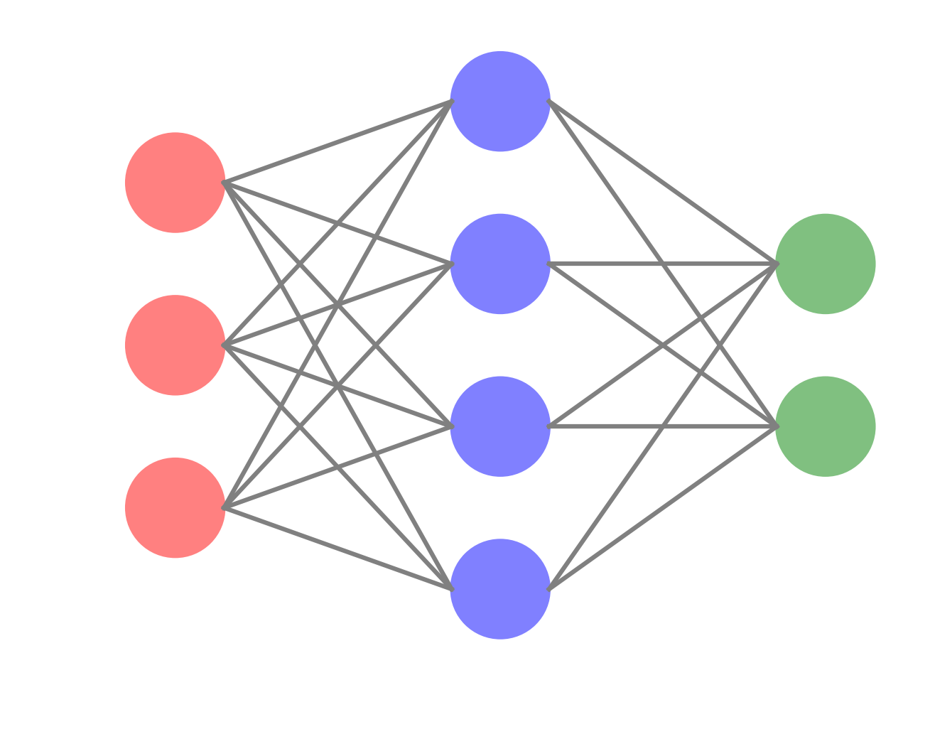
(a function I wrote for generating images of neural network graphs with given number of layers and nodes can be found here).
To demonstrate the feed-forward network, we consider a network with one hidden layer (the smallest possible deep neural network). We also use vectorized form for the equations in order to simplify notation and allow for efficient implementation.
The input layer is column vector of size $n_{input}$, next we have a hidden layer with $n_{h}$ nodes. The hidden layer is connected to the inputs with a weight matrix $W_{h}$ of size $n_{h}\times n_{input}$, such that $W^{h}{ij}$ is the weight connecting input node $i$ to hidden note $j$. Additionally we have a bias vector ${\bf b}{h}$ of size $n_{h}$ for the hidden layer. Finally, we have an output layer with $n_{output}$ nodes, which can denote either different classes in a supervised classification problem, or real values in a regression type problem. The output layer is similarly connected to the hidden layer with a weight matrix $W_{o}$ of size $n_{o}\times n_{h}$, and a bias vector ${\bf b}_{o}$ for the output nodes of size.
\[z_{h}=W_{h}\cdot X_{input}+b_{h}, \quad (n_{h}) \\ a_{h}=f(z_{h}), \\ z_{o} = W_{o}\cdot a_{h}+b_{o}, \quad (n_{o}) \\ a_{o} = f(z_{o}), \quad (n_{o}).\]In parenthesis I give the output dimensions in each step.
Backpropagation
In order to know how a given weight influences the output, which is given by the gradient of the output with respect to a given weight, one therefore needs to go backwards from the output, and chain together the derivatives of the intermediate outputs from each layer. Also known as the chain rule. We start with a loss function $L(W,b)$ which is a function of the weights and biases. The gradient descent minimization process updates the parameters at each learning step according to,
\[W:= W -\eta \nabla_{W}L(W,b) \\ b:= b - \eta \nabla_{b}L(W,b),\]where $\eta$ is the learning rate. To obtain the gradients we employ the chain rule,
\[\frac{\partial L}{\partial W^{o}_{ij}} = \frac{\partial L}{\partial a^{o}_i} \frac{\partial a^{o}_i}{\partial z^{o}_i}\frac{\partial z^{o}_i}{\partial W^{o}_{ij}} = \nabla_{a_{o}} L \times f'(z_{o}) \cdot a_{h}^T, \\ \frac{\partial L}{\partial b_{o}}=\nabla_{a_{o}} L \times f'(z_{o}) \cdot a_{h}^T, \\ \frac{\partial L}{\partial W^{h}_{ij}} = \frac{\partial L}{\partial a^{o}_k} \frac{\partial a^{o}_k}{\partial z^{o}_k}\frac{\partial z^{o}_k}{\partial a_i^{h}}\frac{\partial a_i^{h}}{\partial z_i^{h}}\frac{\partial z_i^{h}}{\partial W_{ij}^{h}}= (\nabla_{a_{o}} L\times f'(z_{o}))\cdot W^T_{o} f'(z_{h})\cdot x^T, \\ \frac{\partial L}{\partial b_{h}}=(\nabla_{a_{o}} L\times f'(z_{o}))\cdot W^T_{o} f'(z_{h}).\]Using a single data point for updating the weights is known as stochastic gradient descent, due to the noisier but faster nature of the updates, alternatively there is batch or mini-batch gradient descent, where the input contains several data points forming an input matrix of size $n_{input}\times n_{data}$, which is closer to the true gradient of the loss but is more expensive computationally. (a stack exchange answer on pros and cons of the two limits.)
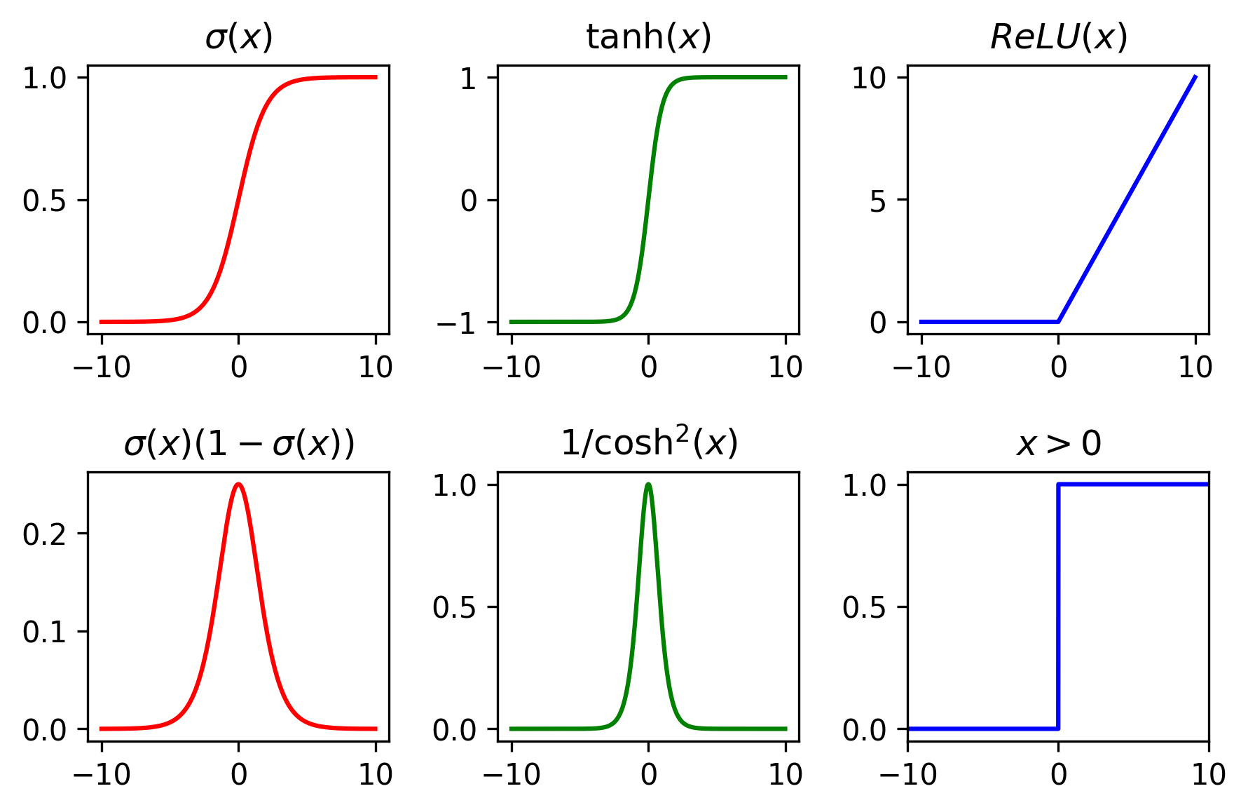
A few common non-linear activation functions are the sigmoid, tanh, and relu. Note from the backpropagation equations that the learning depends on the derivatives of the activation functions. Below I show the activations functions and their derivatives.
Two common loss functions are the mean square error and the cross entropy given for a single sample by,
\[L_2=\frac{1}{2} \sum_j (y_j- a^o_j)^2, \\ L_c=-\sum_j^{n_o}[y_j \log(a^o_j)+(1-y_j)\log(1-a_j^o)],\]where $y_j$ denotes the true value for node $j$, and $a_o$ the network’s output.
The backpropagation requires the gradients of the cost function with respect to the weights and biases. In particular we need the derivative with respect to the output,
\[\frac{\partial L_2}{\partial a^o_j}\frac{\partial a_j^o}{\partial z^o_j} = (y_j-a_j^o)f'(z^o_j), \\ \frac{\partial L_c}{\partial a^o_j}\frac{\partial a^o_j}{\partial z^o_j} = \frac{y_j-a^o_j}{a^o_j(1-a^o_j)}f'(z^o_j)=(a^o_j-y_j),\]where in the second row we assumed a sigmoid activation in the output layer, satisfying (see below) $f’(z^o_j) = a^o_j(1-a^o_j)$. Note, that in the second case, the gradient depends only the error as opposed to the derivative of the activation function in the first case. This makes the learning faster and prevents neurons from getting saturated and stop learning. Additionally, when considering multi-class classification problems the output layer activation is replaced by a soft-max layer
\[\frac{e^{z_{out}}}{\sum_{c} {e^{z_c}}},\]which converts the outputs into a probability distribution. In that case the cross entropy cost is given by
\[L_c = -\sum\limits_j^{classes} y_j\log(a^o_j),\]and the gradients are given by a similar form,
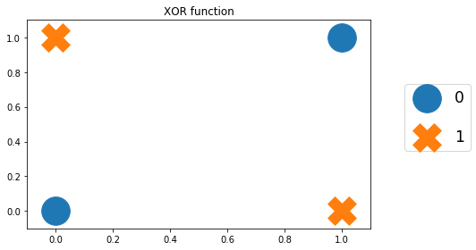
\[\frac{\partial L_c}{\partial a^o_j}\frac{\partial a^o_j}{z^o_i}=a^o_i-y_i.\]A simple but historically important example of using an artificial neural network, is the XOR function, which takes two binary inputs, and outputs zero for (0,0),(1,1) and 1 for (1,0),(0,1). As the two classes (1 or 0) cannot be linearly separated, one needs to use a neural network with a hidden layer. The full ipython notebook can be found here.
XOR function
plt.scatter([0,1],[0,1],s=1000,marker='o',label='0')
plt.scatter([0,1],[1,0],s=1000,marker='X',label='1')
plt.legend(loc=(1.1,0.37),fontsize = 'xx-large',labelspacing=1.5)
plt.title('XOR function')
plt.xlim([-0.1,1.1])
plt.ylim([-0.1,1.1]);
plt.tight_layout()
Neural network class
  class neural_network:

    def __init__(self,ni,nh,no,activation, lr):
        self.ni = ni
        self.nh = nh
        self.no = no
        self.lr = lr
        self.activation = activation

        #self.wh=np.random.rand(self.nh,self.ni)
        self.wh = np.random.normal(0, 1, (self.nh, self.ni))/np.sqrt(ni)
        self.bh=np.zeros((self.nh,1))
        #self.wo=np.random.rand(self.no,self.nh)
        self.wo = np.random.normal(0, 1, (self.no, self.nh))/np.sqrt(nh)
        self.bo=np.zeros((self.no,1))

        if activation=='sigmoid':
            self.nonlin= lambda x: 1/(1+np.exp(-x))
            self.dnonlin= lambda x: 1/(1+np.exp(-x))*(1-1/(1+np.exp(-x)))
        elif activation=='tanh':
            self.nonlin= lambda x: np.tanh(x)
            self.dnonlin= lambda x: 1/np.cosh(x)**2
        else:
            self.nonlin=lambda x: np.maximum(x, 0, x)
            self.dnonlin=lambda x: np.ones(x.shape)*(x>0)

        pass

    def loss(self,y,pred):
        return np.sum(0.5*(y-pred)**2)

    def predict(self,x):
        x=x.T
        a1=self.nonlin(np.dot(self.wh,x)+self.bh)
        a2=self.nonlin(np.dot(self.wo,a1)+self.bo)
        return a2

    def train(self,X,y):

        X=X.T
        y=y.T


        #train using the whole training sample
        batch_size = X.shape[1]

        #number of times to go over the training data
        epochs=50000

        print('training network with ' + self.activation + ' activation:')
        for i in range(epochs):
            #input into hidden layer
            zh=np.dot(self.wh,X)+np.repeat(self.bh,batch_size,axis=1)
            #hidden layer activations
            ah=self.nonlin(zh)
            #input into output layer
            zo=np.dot(self.wo,ah)+np.repeat(self.bo,batch_size,axis=1)
            #output layer
            ao=self.nonlin(zo)

            #output layer error - difference with true label y
            err=(ao-y)

            #print error every 10000 epochs
            if (i%10000==0):
                print('loss after %d epochs %f' % (i,self.loss(y,ao)))

            delo=err*self.dnonlin(zo)
            delh=(self.wo.T.dot(delo))*self.dnonlin(zh)

            #weights update
            self.wh-=self.lr*np.dot(delh,X.T)/batch_size
            self.wo-=self.lr*np.dot(delo,ah.T)/batch_size

            #biases update
            meanh=np.expand_dims(np.sum(delh,axis=1)/batch_size,1)
            meano=np.expand_dims(np.sum(delo,axis=1)/batch_size,1)
            self.bh-=self.lr*meanh
            self.bo-=self.lr*meano

        pass
setting up network and learning
np.random.seed(0)

X=np.array([[0,0],[1,0],[0,1],[1,1]])
y=np.array([[0],[1],[1],[0]])

nn1=neural_network(2,2,1,'sigmoid',5)
nn2=neural_network(2,2,1,'tanh',0.3)
nn3=neural_network(2,2,1,'relu',0.1)

nn1.train(X,y)
print()
nn2.train(X,y)
print()
nn3.train(X,y)
training network with sigmoid activation:
loss after 0 epochs 0.524041
loss after 10000 epochs 0.000211
loss after 20000 epochs 0.000101
loss after 30000 epochs 0.000066
loss after 40000 epochs 0.000049

training network with tanh activation:
loss after 0 epochs 0.815223
loss after 10000 epochs 0.000089
loss after 20000 epochs 0.000041
loss after 30000 epochs 0.000026
loss after 40000 epochs 0.000019

training network with relu activation:
loss after 0 epochs 0.726709
loss after 10000 epochs 0.000000
loss after 20000 epochs 0.000000
loss after 30000 epochs 0.000000
loss after 40000 epochs 0.000000
Check final network results
print('sigmoid net:')
for x,p in zip(X,nn1.predict(X)[0]):
    print('input :',x, 'output:', p)

print('tanh net:')
for x,p in zip(X,nn2.predict(X)[0]):
    print('input :',x, 'output:', p)

print('relu net:')
for x,p in zip(X,nn3.predict(X)[0]):
    print('input :',x, 'output:', p)
sigmoid net:
input : [0 0] output: 0.00498677608341
input : [1 0] output: 0.995797811796
input : [0 1] output: 0.995807280359
input : [1 1] output: 0.00427497259731
tanh net:
input : [0 0] output: 2.54374979424e-05
input : [1 0] output: 0.996137582397
input : [0 1] output: 0.996104441828
input : [1 1] output: 3.76155213167e-05
relu net:
input : [0 0] output: 4.20935895214e-15
input : [1 0] output: 1.0
input : [0 1] output: 1.0
input : [1 1] output: 1.78584538084e-15
Digits classification
The ‘hello world’ problem of deep learning is
the classification of handwritten digits.
Below are some examples from the MNIST dataset,
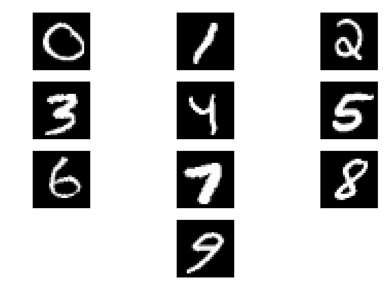
A completely random guess indicating no learning has been done would have an average accuracy of $10%$. Therefore to show that learning has been achieved on previously unseen data, requires a significantly higher accuracy. The ipython notebook with the code can be found here.
The neural network class with the soft max layer and the cross entropy cost function is given below. Additionally to control overfitting we include a regularization term, which aims at keeping the weights values small.
\[L_2 = \frac{\mu}{2n}\sum_W W^2\]such that the modification to the gradient of the weights is simply $\frac{1}{n}\mu W$.
class neural_network:

    def __init__(self,ni,nh,no,activation,lr,ll):
        self.ni = ni
        self.nh = nh
        self.no = no
        self.lr = lr
        self.activation = activation
        self.reg = ll

        np.random.seed(0)
        self.wh = np.random.normal(0, 1, (self.nh, self.ni))/np.sqrt(ni)
        self.bh=np.zeros((self.nh,1))
        self.wo = np.random.normal(0, 1, (self.no, self.nh))/np.sqrt(nh)
        self.bo=np.zeros((self.no,1))

        if activation=='sigmoid':
            self.nonlin= lambda x: 1/(1+np.exp(-x))
            self.dnonlin= lambda x: 1/(1+np.exp(-x))*(1-1/(1+np.exp(-x)))
        elif activation=='tanh':
            self.nonlin= lambda x: np.tanh(x)
            self.dnonlin= lambda x: 1/np.cosh(x)**2
        else:
            self.nonlin=lambda x: np.maximum(x, 0, x)
            self.dnonlin=lambda x: np.ones(x.shape)*(x>0)

        pass

    def loss(self,y,pred):
        return np.sum(np.nan_to_num(-y*np.log(pred)))+self.reg/2*(np.sum(self.wh[:]**2)+np.sum(self.wo[:]**2))

    @staticmethod
    def softmax(z):
        sm=np.sum(np.exp(z))
        return np.exp(z)/sm

    def predict(self,x):
        x=np.array(x,ndmin=2).T
        a1=self.nonlin(np.dot(self.wh,x)+self.bh)
        a2=np.dot(self.wo,a1)+self.bo
        o2=self.softmax(a2)
        return o2


    def score(self,X,y):
        score_lst=[]
        for i in range(y.shape[1]):
            pred=np.argmax(self.predict(X[:,i]))
            yv=np.argmax(y[:,i])
            score_lst.append(np.int(pred==yv))

        print('accuracy: ', np.sum(score_lst)/len(score_lst))
        # return list of scores
        return score_lst

    def train(self,X,y):

        #train using the whole training sample
        batch_size = 1 #X.shape[1]

        #number of times to go over the training data
        epochs=200

        loss_lst=[]
        print('training network with ' + self.activation + ' activation:')
        for i in range(epochs):
            ls=0
            m=0
            gradwh=0
            gradwo=0
            gradbh=0
            gradbo=0

            for (xi,yi) in zip(X.T,y.T):
                m+=1
                xi=np.array(xi,ndmin=2).T
                yi=np.array(yi,ndmin=2).T
                #input into hidden layer
                zh=np.dot(self.wh,xi)+self.bh
                #hidden layer activations
                ah=self.nonlin(zh)
                #input into output layer
                zo=np.dot(self.wo,ah)+self.bo
                #output layer

                #ao=self.nonlin(zo)
                ao=self.softmax(zo)

                #output layer error - difference with true label y
                err=(ao-yi)

                ls+=(self.loss(yi,ao))

                delo = err

                delh=(self.wo.T.dot(delo))*self.dnonlin(zh)

                gradwh+=np.dot(delh,xi.T)
                gradwo+=np.dot(delo,ah.T)
                gradbh+=delh
                gradbo+=delo

                minibatch=10
                if m%minibatch==0:
                    #weights update
                    self.wh-=self.lr*(gradwh)/minibatch+self.lr*self.reg*self.wh
                    self.wo-=self.lr*(gradwo)/minibatch+self.lr*self.reg*self.wo

                    #biases update
                    self.bh-=self.lr*gradbh/minibatch
                    self.bo-=self.lr*gradbo/minibatch

                    gradwh=0
                    gradwo=0
                    gradbh=0
                    gradbo=0

            loss_lst.append(ls)
            if (i%10==0):
                print('epoch: ',i,', loss: ',ls)

        plt.plot(loss_lst)
        plt.show()

        pass
I create an instance of the neural network class, with $784$ input nodes representing the $8\times 28$ pixels in the grayscale image of a digit. 100 hidden layer nodes, and 10 output nodes for the 10 digits. I use ReLU activation, 0.1 learning rate and 0.002 regularization parameter. I split the training set consisting of 20000 samples into 18000 training samples and 2000 validation samples, which allow to tune the hyperparameters such as the learning rate, regularization etc. The model is then tested on a test set with 10000 samples. I then train the network for 200 epochs and minibatch of size 10.
nn1=neural_network(784,100,10,'relu',0.1,0.002)
nn1.train(x_train,y_train)
training network with relu activation:
epoch:  0 , loss:  9408.25257833
epoch:  10 , loss:  4440.39945997
epoch:  20 , loss:  4333.96701063
epoch:  30 , loss:  4277.59876745
epoch:  40 , loss:  4244.73716297
epoch:  50 , loss:  4234.4720515
epoch:  60 , loss:  4224.44056598
epoch:  70 , loss:  4213.89872276
epoch:  80 , loss:  4206.53568999
epoch:  90 , loss:  4195.75618751
epoch:  100 , loss:  4192.46048788
epoch:  110 , loss:  4193.168517
epoch:  120 , loss:  4183.1714839
epoch:  130 , loss:  4178.7188555
epoch:  140 , loss:  4177.35391609
epoch:  150 , loss:  4173.00837802
epoch:  160 , loss:  4175.69934598
epoch:  170 , loss:  4172.88872587
epoch:  180 , loss:  4177.35118544
epoch:  190 , loss:  4173.31381838
The loss as a function of epoch number

print('train set:')
train_score=nn1.score(x_train,y_train)
print('validation set:')
val_score=nn1.score(x_val,y_val)
print('test set:')
test_score=nn1.score(x_test,y_test)
train set:
accuracy:  0.983166666667
validation set:
accuracy:  0.963
test set:
accuracy:  0.9649
I get a test set accuracy of 96.5%.