Kelly Criterion
The Kelly criterion answers the question: what is the optimal fraction of capital to allocate given an edge in a a repeated trading setting?
Since the wealth evolves by multiplication (compounds) one should maximize the expected long term growth rate as opposed to the expected return.
$W_T = W_0 \Pi_{t=1}^{T} (1+fR_t)$
where, $W_t$ = wealth, $f$ = fraction of wealth allocated, $R_t$ = return per unit capital in period $t$t.
This is the main insight and innovation in the criteria. If we were to simply maximize expected wealth after one period: $W_0 E[1 + fR]$, we would simply bet as much as possible, as the expectation is linear in the return ($R$). But for repeated betting, this doesn’t take into account the path and the compounding, which can lead to ruin. For example: making +50%, then -50%, average return is 0, but wealth is $(1.5)(0.5) = 0.75$ of original wealth.
Taking log of the wealth compounding formula:
$\frac{1}{T}\log W_T/W_0 = \frac{1}{T} \sum_{t=1}^T \log(1+fR_t)$
Under repeated bets, the right hand side goes to the expected value of the growth rate.
Binary Kelly
In a binary trade we have: $p$: win probability, $q=1-p$: loss probability, $b$ = payout odds per unit staked (win $b$ per 1 bet, lose 1 per 1 bet).
The expected log growth: $g(f) = p \log(1+fb) + q\log(1-f)$, maximizing: $ \frac{pb}{1+fb} = \frac{1}{1-f}$
$f^* = \frac{pb - q}{b}$
The numerator is actually the expected return.
A special case is equal money for winning or losing. In this case $b=1$, which simplifies the Kelly fraction to: $f^* = 2p - 1$.
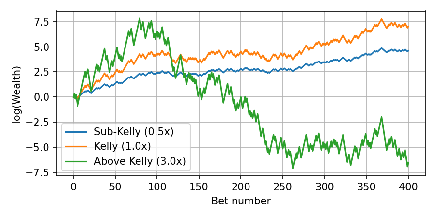
Simulated log wealth example: $p=0.55, b=1.1$ using sub Kelly, Kelly, and above Kelly.
Kelly in markets
In markets, returns are not binary, but continuous, we need to maximize the log growth: $E(\log(1 + fR))$, where R is the return per period.
As an approximation, assuming $R\lt\lt 1$, we expend the log using Taylor series:
$ E (\log(1 + fR)) \approx E(fR - \frac{1}{2}f^2R^2) = f\mu - \frac{1}{2}f^2 \sigma^2$
The maximal expected growth is then:
$ f^* = \frac{\mu}{\sigma^2} $.
This is basically the Sharpe ratio divided by $\sigma$.
In practice, as we don’t have full knowledge of our edge or future return, people typically use a fractional-Kelly approach, e.g. using half-Kelly.